Now we can use sparktools by beta version in GATK4, but it is not for commercial since the result is not same with non-spark. So When can we used it for commercial? Do you have any plan?
THX.
↧
【GATK4 SPARK】When the sparktool can be released in GATK4?
↧
HaplotypeCaller: Alternate allele get called or not depending on -ip option
Hi, I'm currently analyzing some data (exome-seq) using HaplotypeCaller and get what seems to me an odd behaviour:
The problem is that I've got a position which is clearly bi-allelic in IGV and that is said to have only the reference allele in the gVCF I'm generating with HaplotypeCaller.
Here is the command line I used:
nohup java -jar PATH/GenomeAnalysisTK-3.4-46/GenomeAnalysisTK.jar \
-T HaplotypeCaller \
-R PATH/ucsc.hg19_noHaps.fasta \
-I PATH/JLCL254.realigned.recalibrated.bam \
-L PATH/merged.bed \
-ip 50 \
--emitRefConfidence GVCF \
--variant_index_type LINEAR \
--variant_index_parameter 128000 \
-o JLCL254.vcf
Here is the gVCF line of the variant of interest:
CHROM POS ID REF ALT QUAL FILTER INFO FORMAT JLCL254
chr1 912049 . T NON_REF . . END=912049 GT:DP:GQ:MIN_DP:PL 0/0:68:0:68:0,0,0
The variant of interest is located 19bp away from the captured region but with "-ip 50" it should be detected.
To check what is really analyzed, I output the bamout for all analyzed regions (-L PATH/merged.bed) and saw that the location of the variant is not analyzed (If I'm correct: as there is no coverage, this is not an active region).
Then I forced the bamout at the location +/-20nt around my variant to check whether some reads with the alternate allele are still kept. I used:
-L chr1:912029-912069 \
-forceActive \
-disableOptimizations
Doing so I've being able to see that many reads with the alternate allele are indeed still kept. The gVCF file generated along with the bamout file contains now my variant of interest with the alternate allele:
CHROM POS ID REF ALT QUAL FILTER INFO FORMAT JLCL254
chr1 912049 rs9803103 T C,NON_REF 1235.77 . BaseQRankSum=-0.677;ClippingRankSum=-0.942;DB;DP=61;MLEAC=1,0;MLEAF=0.500,0.00;MQ=54.88;MQRankSum=-0.600;ReadPosRankSum=-0.195 GT:AD:DP:GQ:PL:SB 0/1:19,42,0:61:99:1264,0,448,1321,574,1895:3,16,6,36
Please see an IGV screenshot:

Tracks are (from top to bottom):
* the original bam file
* the bamout for all captured regions (known from the file -L PATH/merged.bed)
* the forced bamout (at the location of the variant i.e -L chr1:912029-912069)
* merged.bed is the file used with the -L option.
Finally, I tried to call variants changing the -ip option to 100 and got the alternate allele called.
Please note that:
If I manually add/subtract 50bp to the closest target region boundaries, I've got the same result as with -ip 50.
If I manually add/subtract 100bp to the closest target region boundaries, I've got the same result as with -ip 100.
I tried several versions of GATK (3.46, 3.7, 4.0.4.0) and always got the same results.
I may have miss something but so far I can't explain myself what's happening. Do you see any explanation for what I observe? Do you see any options I should use to overcome this?
Many thanks in advance for your help.
NB: java -version
openjdk version "1.8.0_171"
OpenJDK Runtime Environment (build 1.8.0_171-b10)
OpenJDK 64-Bit Server VM (build 25.171-b10, mixed mode)
↧
↧
How MuTect identifies candidate somatic mutations
Please note that this article refers to the original standalone version of MuTect. A new version is now available within GATK (starting at GATK 3.5) under the name MuTect2. This new version is able to call both SNPs and indels. See the GATK version 3.5 release notes and the MuTect2 tool documentation for further details.
Overview
In a nutshell, the MuTect analysis consists of three steps:
- Pre-processing the aligned reads in the tumor and normal sequencing data
- Statistical analysis to identify sites that are likely to carry somatic mutations with high confidence
- Post-processing of candidate somatic mutations
This document summarizes the key points of these three steps. For complete details, please see the 2013 publication in Nature Biotechnology:
1. Pre-processing the aligned reads in the tumor and normal sequencing data
In this step we ignore reads with too many mismatches or very low quality scores since these represent noisy reads that introduce more noise than signal.
2. Statistical analysis to identify sites that are likely to carry somatic mutations with high confidence
The statistical analysis predicts a somatic mutation by using two Bayesian classifiers – the first aims to detect whether the tumor is non-reference at a given site and, for those sites that are found as non-reference, the second classifier makes sure the normal does not carry the variant allele. In practice the classification is performed by calculating a LOD score (log odds) and comparing it to a cutoff determined by the log ratio of prior probabilities of the considered events.
For the tumors we calculate:
$$ LOD_T = log_{10} \left ( \frac{ P( \text{observed data in tumor | site is mutated} ) } { P( \text{observed data in tumor | site is reference} ) } \right ) $$
And for the normal:
$$ LOD_N = log_{10} \left ( \frac{ P( \text{observed data in normal | site is reference} ) } { P( \text{observed data in normal | site is mutated} ) } \right ) $$
Since we expect somatic mutations to occur at a rate of ~1 per Mb, we require
$$ LOD_T > log_{10} (0.5 \times 10^{-6} ) \approx 6.3 $$
which guarantees that our false positive rate, due to noise in the tumor, is less than half of the somatic mutation rate.
In the normal, for sites that are not in dbSNP, we require
$$ LOD_N > log_{10} (0.5 \times 10^{-2} ) \approx 2.3 $$
since non-dbSNP germline variants occur roughly at a rate of 100 per Mb. This cutoff guarantees that the false positive somatic call rate, due to missing the variant in the normal, is also less than half the somatic mutation rate.
3. Post-processing of candidate somatic mutations
This step aims to eliminate artifacts of next-generation sequencing, short read alignment and hybrid capture. For example, sequence context can cause hallucinated alternate alleles but often only in a single direction. Therefore, we test that the alternate alleles supporting the mutations are observed in both directions.
Note on method validation
Most cancer genome studies at the Broad Institute have made use of MuTect and have validated the mutation calls as a part of their cancer biology papers, showing that MuTect has a very low false positive rate. A summary of validation rates from these papers are show below:

↧
(How to) Map reads to a reference with alternate contigs like GRCh38
Document is in BETA. It may be incomplete and/or inaccurate. Post suggestions to the Comments section and be sure to read about updates also within the Comments section.
 This exploratory tutorial provides instructions and example data to map short reads to a reference genome with alternate haplotypes. Instructions are suitable for indexing and mapping reads to GRCh38.
► If you are unfamiliar with terms that describe reference genome components, or GRCh38 alternate haplotypes, take a few minutes to study the Dictionary entry Reference Genome Components.
► For an introduction to GRCh38, see Blog#8180.
Specifically, the tutorial uses BWA-MEM to index and map simulated reads for three samples to a mini-reference composed of a GRCh38 chromosome and alternate contig (sections 1–3). We align in an alternate contig aware (alt-aware) manner, which we also call alt-handling. This is the main focus of the tutorial.
The decision to align to a genome with alternate haplotypes has implications for variant calling. We discuss these in section 5 using the callset generated with the optional tutorial steps outlined in section 4. Because we strategically placed a number of SNPs on the sequence used to simulate the reads, in both homologous and divergent regions, we can use the variant calls and their annotations to examine the implications of analysis approaches. To this end, the tutorial fast-forwards through pre-processing and calls variants for a trio of samples that represents the combinations of the two reference haplotypes (the PA and the ALT). This first workflow (tutorial_8017) is suitable for calling variants on the primary assembly but is insufficient for capturing variants on the alternate contigs.
For those who are interested in calling variants on the alternate contigs, we also present a second and a third workflow in section 6. The second workflow (tutorial_8017_toSE) takes the processed BAM from the first workflow, makes some adjustments to the reads to maximize their information, and calls variants on the alternate contig. This approach is suitable for calling on ~75% of the non-HLA alternate contigs or ~92% of loci with non-HLA alternate contigs (see table in section 6). The third workflow (tutorial_8017_postalt) takes the alt-aware alignments from the first workflow and performs a postalt-processing step as well as the same adjustment from the second workflow. Postalt-processing uses the bwa-postalt.js javascript program that Heng Li provides as a companion to BWA. This allows for variant calling on all alternate contigs including HLA alternate contigs.
The tutorial ends by comparing the difference in call qualities from the multiple workflows for the given example data and discusses a few caveats of each approach.
► The three workflows shown in the diagram above are available as WDL scripts in our GATK Tutorials WDL scripts repository.
Jump to a section
- Index the reference FASTA for use with BWA-MEM
- Include the reference ALT index file
☞ What happens if I forget the ALT index file? - Align reads with BWA-MEM
☞ How can I tell if a BAM was aligned with alt-handling?
☞ What is thepatag? - (Optional) Add read group information, preprocess to make a clean BAM and call variants
- How can I tell whether I should consider an alternate haplotype for a given sample?
(5.1) Discussion of variant calls for tutorial_8017 - My locus includes an alternate haplotype. How can I call variants on alt contigs?
(6.1) Variant calls for tutorial_8017_toSE
(6.2) Variant calls for tutorial_8017_postalt - Related resources
Tools involved
BWA v0.7.13 or later releases. The tutorial uses v0.7.15.
Download from here and see Tutorial#2899 for installation instructions.
Thebwa-postalt.jsscript is within thebwakitfolder.Picard tools v2.5.0 or later releases. The tutorial uses v2.5.0.
- Optional GATK tools. The tutorial uses v3.6.
- Optional Samtools. The tutorial uses v1.3.1.
- Optional Gawk, an AWK-like tool that can interpret bitwise SAM flags. The tutorial uses v4.1.3.
- Optional k8 Javascript shell. The tutorial uses v0.2.3 downloaded from here.
Download example data
Download tutorial_8017.tar.gz, either from the GoogleDrive or from the ftp site. To access the ftp site, leave the password field blank. The data tarball contains the paired FASTQ reads files for three samples. It also contains a mini-reference chr19_chr19_KI270866v1_alt.fasta and corresponding .dict dictionary, .fai index and six BWA indices including the .alt index. The data tarball includes the output files from the workflow that we care most about. These are the aligned SAMs, processed and indexed BAMs and the final multisample VCF callsets from the three presented workflows.
 The mini-reference contains two contigs subset from human GRCh38:
 chr19 and chr19_KI270866v1_alt. The ALT contig corresponds to a diverged haplotype of chromosome 19. Specifically, it corresponds to chr19:34350807-34392977, which contains the glucose-6-phosphate isomerase or GPI gene. Part of the ALT contig introduces novel sequence that lacks a corresponding region in the primary assembly.
Using instructions in Tutorial#7859, we simulated paired 2x151 reads to derive three different sample reads that when aligned give roughly 35x coverage for the target primary locus. We derived the sequences from either the 43 kbp ALT contig (sample ALTALT), the corresponding 42 kbp region of the primary assembly (sample PAPA) or both (sample PAALT). Before simulating the reads, we introduced four SNPs to each contig sequence in a deliberate manner so that we can call variants.
► Alternatively, you may instead use the example input files and commands with the full GRCh38 reference. Results will be similar with a handful of reads mapping outside of the mini-reference regions.
1. Index the reference FASTA for use with BWA-MEM
Our example chr19_chr19_KI270866v1_alt.fasta reference already has chr19_chr19_KI270866v1_alt.dict dictionary and chr19_chr19_KI270866v1_alt.fasta.fai index files for use with Picard and GATK tools. BWA requires a different set of index files for alignment. The command below creates five of the six index files we need for alignment. The command calls the index function of BWA on the reference FASTA.
bwa index chr19_chr19_KI270866v1_alt.fasta
This gives .pac, .bwt, .ann, .amb and .sa index files that all have the same chr19_chr19_KI270866v1_alt.fasta basename. Tools recognize index files within the same directory by their identical basename. In the case of BWA, it uses the basename preceding the .fasta suffix and searches for the index file, e.g. with .bwt suffix or .64.bwt suffix. Depending on which of the two choices it finds, it looks for the same suffix for the other index files, e.g. .alt or .64.alt. Lack of a matching .alt index file will cause BWA to map reads without alt-handling. More on this next.
Note that the .64. part is an explicit indication that index files were generated with version 0.6 or later of BWA and are the 64-bit indices (as opposed to files generated by earlier versions, which were 32-bit). This .64. signifier can be added automatically by adding -6 to the bwa index command.
2. Include the reference ALT index file
Be sure to place the tutorial's mini-ALT index file chr19_chr19_KI270866v1_alt.fasta.alt with the other index files. Also, if it does not already match, change the file basename to match. This is the sixth index file we need for alignment. BWA-MEM uses this file to prioritize primary assembly alignments for reads that can map to both the primary assembly and an alternate contig. See BWA documentation for details.
- As of this writing (August 8, 2016), the SAM format ALT index file for GRCh38 is available only in the x86_64-linux bwakit download as stated in this bwakit README. The
hs38DH.fa.altfile is in theresource-GRCh38folder. - In addition to mapped alternate contig records, the ALT index also contains decoy contig records as unmapped SAM records. This is relevant to the postalt-processing we discuss in section 6.2. As such, the postalt-processing in section 6 also requires the ALT index.
For the tutorial, we subset from hs38DH.fa.alt to create a mini-ALT index, chr19_chr19_KI270866v1_alt.fasta.alt. Its contents are shown below.

The record aligns the chr19_KI270866v1_alt contig to the chr19 locus starting at position 34,350,807 and uses CIGAR string nomenclature to indicate the pairwise structure. To interpret the CIGAR string, think of the primary assembly as the reference and the ALT contig sequence as the read. For example, the 11307M at the start indicates 11,307 corresponding sequence bases, either matches or mismatches. The 935S at the end indicates a 935 base softclip for the ALT contig sequence that lacks corresponding sequence in the primary assembly. This is a region that we consider highly divergent or novel. Finally, notice the NM tag that notes the edit distance to the reference.
☞ What happens if I forget the ALT index file?
If you omit the ALT index file from the reference, or if its naming structure mismatches the other indexes, then your alignments will be equivalent to the results you would obtain if you run BWA-MEM with the -j option. The next section gives an example of what this looks like.
3. Align reads with BWA-MEM
The command below uses an alt-aware version of BWA and maps reads using BWA's maximal exact match (MEM) option. Because the ALT index file is present, the tool prioritizes mapping to the primary assembly over ALT contigs. In the command, the tutorial's chr19_chr19_KI270866v1_alt.fasta serves as reference; one FASTQ holds the forward reads and the other holds the reverse reads.
bwa mem chr19_chr19_KI270866v1_alt.fasta 8017_read1.fq 8017_read2.fq > 8017_bwamem.sam
The resulting file 8017_bwamem.sam contains aligned read records.
- BWA preferentially maps to the primary assembly any reads that can align equally well to the primary assembly or the ALT contigs as well as any reads that it can reasonably align to the primary assembly even if it aligns better to an ALT contig. Preference is given by the primary alignment record status, i.e. not secondary and not supplementary. BWA takes the reads that it cannot map to the primary assembly and attempts to map them to the alternate contigs. If a read can map to an alternate contig, then it is mapped to the alternate contig as a primary alignment. For those reads that can map to both and align better to the ALT contig, the tool flags the ALT contig alignment record as supplementary (0x800). This is what we call alt-aware mapping or alt-handling.
- Adding the
-joption to the command disables the alt-handling. Reads that can map multiply are given low or zero MAPQ scores.

☞ How can I tell if a BAM was aligned with alt-handling?
There are two approaches to this question.
First, you can view the alignments on IGV and compare primary assembly loci with their alternate contigs. The IGV screenshots to the right show how BWA maps reads with (top) or without (bottom) alt-handling.
Second, you can check the alignment SAM. Of two tags that indicate alt-aware alignment, one will persist after preprocessing only if the sample has reads that can map to alternate contigs. The first tag, the AH tag, is in the BAM header section of the alignment file, and is absent after any merging step, e.g. merging with MergeBamAlignment. The second tag, the pa tag, is present for reads that the aligner alt-handles. If a sample does not contain any reads that map equally or preferentially to alternate contigs, then this tag may be absent in a BAM even if the alignments were mapped in an alt-aware manner.
Here are three headers for comparison where only one indicates alt-aware alignment.
File header for alt-aware alignment. We use this type of alignment in the tutorial.
Each alternate contig's @SQ line in the header will have an AH:* tag to indicate alternate contig handling for that contig. This marking is based on the alternate contig being listed in the .alt index file and alt-aware alignment.

File header for -j alignment (alt-handling disabled) for example purposes. We do not perform this type of alignment in the tutorial.
Notice the absence of any special tags in the header.

File header for alt-aware alignment after merging with MergeBamAlignment. We use this step in the next section.
Again, notice the absence of any special tags in the header.

☞ What is the pa tag?
For BWA v0.7.15, but not v0.7.13, ALT loci alignment records that can align to both the primary assembly and alternate contig(s) will have a pa tag on the primary assembly alignment. For example, read chr19_KI270866v1_alt_4hetvars_26518_27047_0:0:0_0:0:0_931 of the ALTALT sample has five alignment records only three of which have the pa tag as shown below.

A brief description of each of the five alignments, in order:
- First in pair, primary alignment on the primary assembly; AS=146, pa=0.967
- First in pair, supplementary alignment on the alternate contig; AS=151
- Second in pair, primary alignment on the primary assembly; AS=120; pa=0.795
- Second in pair, supplementary alignment on the primary assembly; AS=54; pa=0.358
- Second in pair, supplementary alignment on the alternate contig; AS=151
The pa tag measures how much better a read aligns to its best alternate contig alignment versus its primary assembly (pa) alignment. Specifically, it is the ratio of the primary assembly alignment score over the highest alternate contig alignment score. In our example we have primary assembly alignment scores of 146, 120 and 54 and alternate contig alignment scores of 151 and again 151. This gives us three different pa scores that tag the primary assembly alignments: 146/151=0.967, 120/151=0.795 and 54/151=0.358.
In our tutorial's workflow, MergeBamAlignment may either change an alignment's pa score or add a previously unassigned pa score to an alignment. The result of this is summarized as follows for the same alignments.
- pa=0.967 --MergeBamAlignment--> same
- none --MergeBamAlignment--> assigns pa=0.967
- pa=0.795 --MergeBamAlignment--> same
- pa=0.358 --MergeBamAlignment--> replaces with pa=0.795
- none --MergeBamAlignment--> assigns pa=0.795
If you want to retain the BWA-assigned pa scores, then add the following options to the workflow commands in section 4.
- For RevertSam, add
ATTRIBUTE_TO_CLEAR=pa. - For MergeBamAlignment, add
ATTRIBUTES_TO_RETAIN=pa.
In our sample set, after BWA-MEM alignment ALTALT has 1412 pa-tagged alignment records, PAALT has 805 pa-tagged alignment records and PAPA has zero pa-tagged records.
4. Add read group information, preprocess to make a clean BAM and call variants
The initial alignment file is missing read group information. One way to add that information, which we use in production, is to use MergeBamAlignment. MergeBamAlignment adds back read group information contained in an unaligned BAM and adjusts meta information to produce a clean BAM ready for pre-processing (see Tutorial#6483 for details on our use of MergeBamAlignment). Given the focus here is to showcase BWA-MEM's alt-handling, we refrain from going into the details of all this additional processing. They follow, with some variation, the PairedEndSingleSampleWf pipeline detailed here.
Remember these are simulated reads with simulated base qualities. We simulated the reads in a manner that only introduces the planned mismatches, without any errors. Coverage is good at roughly 35x. All of the base qualities for all of the reads are at I, which is, according to this page and this site, an excellent base quality score equivalent to a Sanger Phred+33 score of 40. We can therefore skip base quality score recalibration (BQSR) since the reads are simulated and the dataset is not large enough for recalibration anyway.
Here are the commands to obtain a final multisample variant callset. The commands are given for one of the samples. Process each of the three samples independently in the same manner [4.1–4.6] until the last GenotypeGVCFs command [4.7].
[4.1] Create unmapped uBAM
java -jar picard.jar RevertSam \
    I=altalt_bwamem.sam O=altalt_u.bam \
    ATTRIBUTE_TO_CLEAR=XS ATTRIBUTE_TO_CLEAR=XA
[4.2] Add read group information to uBAM
java -jar picard.jar AddOrReplaceReadGroups \
    I=altalt_u.bam O=altalt_rg.bam \
    RGID=altalt RGSM=altalt RGLB=wgsim RGPU=shlee RGPL=illumina
[4.3] Merge uBAM with aligned BAM
java -jar picard.jar MergeBamAlignment \
    ALIGNED=altalt_bwamem.sam UNMAPPED=altalt_rg.bam O=altalt_m.bam \
    R=chr19_chr19_KI270866v1_alt.fasta \
    SORT_ORDER=unsorted CLIP_ADAPTERS=false \
    ADD_MATE_CIGAR=true MAX_INSERTIONS_OR_DELETIONS=-1 \
    PRIMARY_ALIGNMENT_STRATEGY=MostDistant \
    UNMAP_CONTAMINANT_READS=false \
    ATTRIBUTES_TO_RETAIN=XS ATTRIBUTES_TO_RETAIN=XA
[4.4] Flag duplicate reads
java -jar picard.jar MarkDuplicates \
    INPUT=altalt_m.bam OUTPUT=altalt_md.bam METRICS_FILE=altalt_md.bam.txt \
    OPTICAL_DUPLICATE_PIXEL_DISTANCE=2500 ASSUME_SORT_ORDER=queryname
[4.5] Coordinate sort, fix NM and UQ tags and index for clean BAM
As of Picard v2.7.0, released October 17, 2016, SetNmAndUqTags is no longer available. Use SetNmMdAndUqTags instead.
set -o pipefail
java -jar picard.jar SortSam \
    INPUT=altalt_md.bam OUTPUT=/dev/stdout SORT_ORDER=coordinate | \
    java -jar $PICARD SetNmAndUqTags \
    INPUT=/dev/stdin OUTPUT=altalt_snaut.bam \
    CREATE_INDEX=true R=chr19_chr19_KI270866v1_alt.fasta
[4.6] Call SNP and indel variants in emit reference confidence (ERC) mode per sample using HaplotypeCaller
java -jar GenomeAnalysisTK.jar -T HaplotypeCaller \
    -R chr19_chr19_KI270866v1_alt.fasta \
    -o altalt.g.vcf -I altalt_snaut.bam \
    -ERC GVCF --max_alternate_alleles 3 --read_filter OverclippedRead \
    --emitDroppedReads -bamout altalt_hc.bam
[4.7] Call genotypes on three samples
java -jar GenomeAnalysisTK.jar -T GenotypeGVCFs \
    -R chr19_chr19_KI270866v1_alt.fasta -o multisample.vcf \
    --variant altalt.g.vcf --variant altpa.g.vcf --variant papa.g.vcf
The altalt_snaut.bam, HaplotypeCaller's altalt_hc.bam and the multisample multisample.vcf are ready for viewing on IGV.
Before getting into the results in the next section, we have minor comments on two filtering options.
In our tutorial workflows, we turn off MergeBamAlignment's UNMAP_CONTAMINANT_READS option. If set to true, 68 reads become unmapped for PAPA and 40 reads become unmapped for PAALT. These unmapped reads are those reads caught by the UNMAP_CONTAMINANT_READS filter and their mates. MergeBamAlignment defines contaminant reads as those alignments that are overclipped, i.e. that are softclipped on both ends, and that align with less than 32 bases. Changing the MIN_UNCLIPPED_BASES option from the default of 32 to 22 and 23 restores all of these reads for PAPA and PAALT, respectively. Contaminants are obviously absent for these simulated reads. And so we set UNMAP_CONTAMINANT_READS to false to disable this filtering.
HaplotypeCaller's --read_filter OverclippedRead option similarly looks for both-end-softclipped alignments, then filters reads aligning with less than 30 bases. The difference is that HaplotypeCaller only excludes the overclipped alignments from its calling and does not remove mapping information nor does it act on the mate of the filtered alignment. Thus, we keep this read filter for the first workflow. However, for the second and third workflows in section 6, tutorial_8017_toSE and tutorial_8017_postalt, we omit the --read_filter Overclipped option from the HaplotypeCaller command. We also omit the --max_alternate_alleles 3 option for simplicity.
5. How can I tell whether I should consider an alternate haplotype?
 We consider this question only for our GPI locus, a locus we know has an alternate contig in the reference. Here we use the term locus in its biological sense to refer to a contiguous genomic region of interest. The three samples give the alignment and coverage profiles shown on the right.
What is immediately apparent from the IGV screenshot is that the scenarios that include the alternate haplotype give a distinct pattern of variant sites to the primary assembly much like a fingerprint. These variants are predominantly heterozygous or homozygous. Looking closely at the 3' region of the locus, we see some alignment coverage anomalies that also show a distinct pattern. The coverage in some of the highly diverged region in the primary assembly drops while in others it increases. If we look at the origin of simulated reads in one of the excess coverage regions, we see that they are from two different regions of the alternate contig that suggests duplicated sequence segments within the alternate locus.
The variation pattern and coverage anomalies on the primary locus suggest an alternate haplotype may be present for the locus. We can then confirm the presence of aligned reads, both supplementary and primary, on the alternate locus. Furthermore, if we count the alignment records for each region, e.g. using samtools idxstats, we see the following metrics.
                        ALT/ALT     PA/ALT     PA/PA
chr19                     10005      10006     10000
chr19_KI270866v1_alt       1407        799         0
The number of alignments on the alternate locus increases proportionately with alternate contig dosage. All of these factors together suggest that the sample presents an alternate haplotype.
5.1 Discussion of variant calls for tutorial_8017
The three-sample variant callset gives 54 sites on the primary locus and two additional on the alternate locus for 56 variant sites. All of the eight SNP alleles we introduced are called, with six called on the primary assembly and two called on the alternate contig. Of the 15 expected genotype calls, four are incorrect. Namely, four PAALT calls that ought to be heterozygous are called homozygous variant. These are two each on the primary assembly and on the alternate contig in the region that is highly divergent.
► Our production pipelines use genomic intervals lists that exclude GRCh38 alternate contigs from variant calling. That is, variant calling is performed only for contigs of the primary assembly. This calling on even just the primary assembly of GRCh38 brings improvements to analysis results over previous assemblies. For example, if we align and call variants for our simulated reads on GRCh37, we call 50 variant sites with identical QUAL scores to the equivalent calls in our GRCh38 callset. However, this GRCh37 callset is missing six variant calls compared to the GRCh38 callset for the 42 kb locus: the two variant sites on the alternate contig and four variant sites on the primary assembly.
Consider the example variants on the primary locus. The variant calls from the primary assembly include 32 variant sites that are strictly homozygous variant in ALTALT and heterozygous variant in PAALT. The callset represents only those reads from the ALT that can be mapped to the primary assembly.
In contrast, the two variants in regions whose reads can only map to the alternate contig are absent from the primary assembly callset. For this simulated dataset, the primary alignments present on the alternate contig provide enough supporting reads that allow HaplotypeCaller to call the two variants. However, these variant calls have lower-quality annotation metrics than for those simulated in an equal manner on the primary assembly. We will get into why this is in section 6.
Additionally, for our PAALT sample that is heterozygous for an alternate haplotype, the genotype calls in the highly divergent regions are inaccurate. These are called homozygous variant on the primary assembly and on the alternate contig when in fact they are heterozygous variant. These calls have lower genotype scores GQ as well as lower allele depth AD and coverage DP. The table below shows the variant calls for the introduced SNP sites. In blue are the genotype calls that should be heterozygous variant but are instead called homozygous variant.

Here is a command to select out the intentional variant sites that uses SelectVariants:
java -jar GenomeAnalysisTK.jar -T SelectVariants \
    -R chr19_chr19_KI270866v1_alt.fasta \
    -V multisample.vcf -o multisample_selectvariants.vcf \
    -L chr19:34,383,500 -L chr19:34,389,485 -L chr19:34,391,800 -L chr19:34,392,600 \
    -L chr19_KI270866v1_alt:32,700 -L chr19_KI270866v1_alt:38,700 \
    -L chr19_KI270866v1_alt:41,700 -L chr19_KI270866v1_alt:42,700 \
    -L chr19:34,383,486 -L chr19_KI270866v1_alt:32,714
6. My locus includes an alternate haplotype. How can I call variants on alt contigs?
If you want to call variants on alternate contigs, consider additional data processing that overcome the following problems.
- Loss of alignments from filtering of overclipped reads.
- HaplotypeCaller's filtering of alignments whose mates map to another contig. Alt-handling produces many of these types of reads on the alternate contigs.
- Zero MAPQ scores for alignments that map to two or more alternate contigs. HaplotypeCaller excludes these types of reads from contributing to evidence for variation.
Let us talk about these in more detail.
Ideally, if we are interested in alternate haplotypes, then we would have ensured we were using the most up-to-date analysis reference genome sequence with the latest patch fixes. Also, whatever approach we take to align and preprocess alignments, if we filter any reads as putative contaminants, e.g. with MergeBamAlignment's option to unmap cross-species contamination, then at this point we would want to fish back into the unmapped reads pool and pull out those reads. Specifically, these would have an SA tag indicating mapping to the alternate contig of interest and an FT tag indicating the reason for unmapping was because MergeBamAlignment's UNMAP_CONTAMINANT_READS option identified them as cross-species contamination. Similarly, we want to make sure not to include HaplotypeCaller's --read_filter OverclippedRead option that we use in the first workflow.
 As section 5.1 shows, variant calls on the alternate contig are of low quality--they have roughly an order of magnitude lower QUAL scores than what should be equivalent variant calls on the primary assembly.
For this exploratory tutorial, we are interested in calling the introduced SNPs with equivalent annotation metrics. Whether they are called on the primary assembly or the alternate contig and whether they are called homozygous variant or heterozygous--let's say these are less important, especially given pinning certain variants from highly homologous regions to one of the loci is nigh impossible with our short reads. To this end, we will use the second workflow shown in the workflows diagram. However, because this solution is limited, we present a third workflow as well.
► We present these workflows solely for exploratory purposes. They do not represent any production workflows.
Tutorial_8017_toSE uses the processed BAM from our first workflow and allows for calling on singular alternate contigs. That is, the workflow is suitable for calling on alternate contigs of loci with only a single alternate contig like our GPI locus. Tutorial_8017_postalt uses the aligned SAM from the first workflow before processing, and requires separate processing before calling. This third workflow allows for calling on all alternate contigs, even on HLA loci that have numerous contigs per primary locus. However, the callset will not be parsimonious. That is, each alternate contig will greedily represent alignments and it is possible the same variant is called for all the alternate loci for a given primary locus as well as on the primary locus. It is up to the analyst to figure out what to do with the resulting calls.
 The reason for the divide in these two workflows is in the way BWA assigns mapping quality scores (MAPQ) to multimapping reads. Postalt-processing becomes necessary for loci with two or more alternate contigs because the shared alignments between the primary locus and alternate loci will have zero MAPQ scores. Postalt-processing gives non-zero MAPQ scores to the alignment records. The table presents the frequencies of GRCh38 non-HLA alternate contigs per primary locus. It appears that ~75% of non-HLA alternate contigs are singular to ~92% of primary loci with non-HLA alternate contigs. In terms of bases on the primary assembly, of the ~75 megabases that have alternate contigs, ~64 megabases (85%) have singular non-HLA alternate contigs and ~11 megabases (15%) have multiple non-HLA alternate contigs per locus. Our tutorial's example locus falls under this majority.
In both alt-aware mapping and postalt-processing, alternate contig alignments have a predominance of mates that map back to the primary assembly. HaplotypeCaller, for good reason, filters reads whose mates map to a different contig. However, we know that GRCh38 artificially represents alternate haplotypes as separate contigs and BWA-MEM intentionally maps these mates back to the primary locus. For comparable calls on alternate contigs, we need to include these alignments in calling. To this end, we have devised a temporary workaround.
6.1 Variant calls for tutorial_8017_toSE
Here we are only aiming for equivalent calls with similar annotation values for the two variants that are called on the alternate contig. For the solution that we will outline, here are the results.

Including the mate-mapped-to-other-contig alignments bolsters the variant call qualities for the two SNPs HaplotypeCaller calls on the alternate locus. We see the AD allele depths much improved for ALTALT and PAALT. Corresponding to the increase in reads, the GQ genotype quality and the QUAL score (highlighted in red) indicate higher qualities. For example, the QUAL scores increase from 332 and 289 to 2166 and 1764, respectively. We also see that one of the genotype calls changes. For sample ALTALT, we see a previous no call is now a homozygous reference call (highlighted in blue). This hom-ref call is further from the truth than not having a call as the ALTALT sample should not have coverage for this region in the primary assembly.
For our example data, tutorial_8017's callset subset for the primary assembly and tutorial_8017_toSE's callset subset for the alternate contigs together appear to make for a better callset.
What solution did we apply? As the workflow's name toSE implies, this approach converts paired reads to single end reads. Specifically, this approach takes the processed and coordinate-sorted BAM from the first workflow and removes the 0x1 paired flag from the alignments. Removing the 0x1 flag from the reads allows HaplotypeCaller to consider alignments whose mates map to a different contig. We accomplish this using a modified script of that presented in Biostars post https://www.biostars.org/p/106668/, indexing with Samtools and then calling with HaplotypeCaller as follows. Note this workaround creates an invalid BAM according to ValidateSamFile. Also, another caveat is that because HaplotypeCaller uses softclipped sequences, any overlapping regions of read pairs will count twice towards variation instead of once. Thus, this step may lead to overconfident calls in such regions.
Remove the 0x1 bitwise flag from alignments
samtools view -h altalt_snaut.bam | gawk '{printf "%s\t", $1; if(and($2,0x1))
{t=$2-0x1}else{t=$2}; printf "%s\t" , t; for (i=3; i<NF; i++){printf "%s\t", $i} ;
printf "%s\n",$NF}'| samtools view -Sb - > altalt_se.bam
Index the resulting BAM
samtools index altalt_se.bam
Call variants in -ERC GVCF mode with HaplotypeCaller for each sample
java -jar GenomeAnalysisTK.jar -T HaplotypeCaller \
    -R chr19_chr19_KI270866v1_alt.fasta \
    -I altalt_se.bam -o altalt_hc.g.vcf \
    -ERC GVCF --emitDroppedReads -bamout altalt_hc.bam
Finally, use GenotypeGVCFs as shown in section 4's command [4.7] for a multisample variant callset. Tutorial_8017_toSE calls 68 variant sites--66 on the primary assembly and two on the alternate contig.
6.2 Variant calls for tutorial_8017_postalt
BWA's postalt-processing requires the query-grouped output of BWA-MEM. Piping an alignment step with postalt-processing is possible. However, to be able to compare variant calls from an identical alignment, we present the postalt-processing as an add-on workflow that takes the alignment from the first workflow.
The command uses the bwa-postalt.js script, which we run through k8, a Javascript execution shell. It then lists the ALT index, the aligned SAM altalt.sam and names the resulting file > altalt_postalt.sam.
k8 bwa-postalt.js \
    chr19_chr19_KI270866v1_alt.fasta.alt \
    altalt.sam > altalt_postalt.sam
 The resulting postalt-processed SAM,
 altalt_postalt.sam, undergoes the same processing as the first workflow (commands 4.1 through 4.7) except that (i) we omit --max_alternate_alleles 3 and --read_filter OverclippedRead options for the HaplotypeCaller command like we did in section 6.1 and (ii) we perform the 0x1 flag removal step from section 6.1.
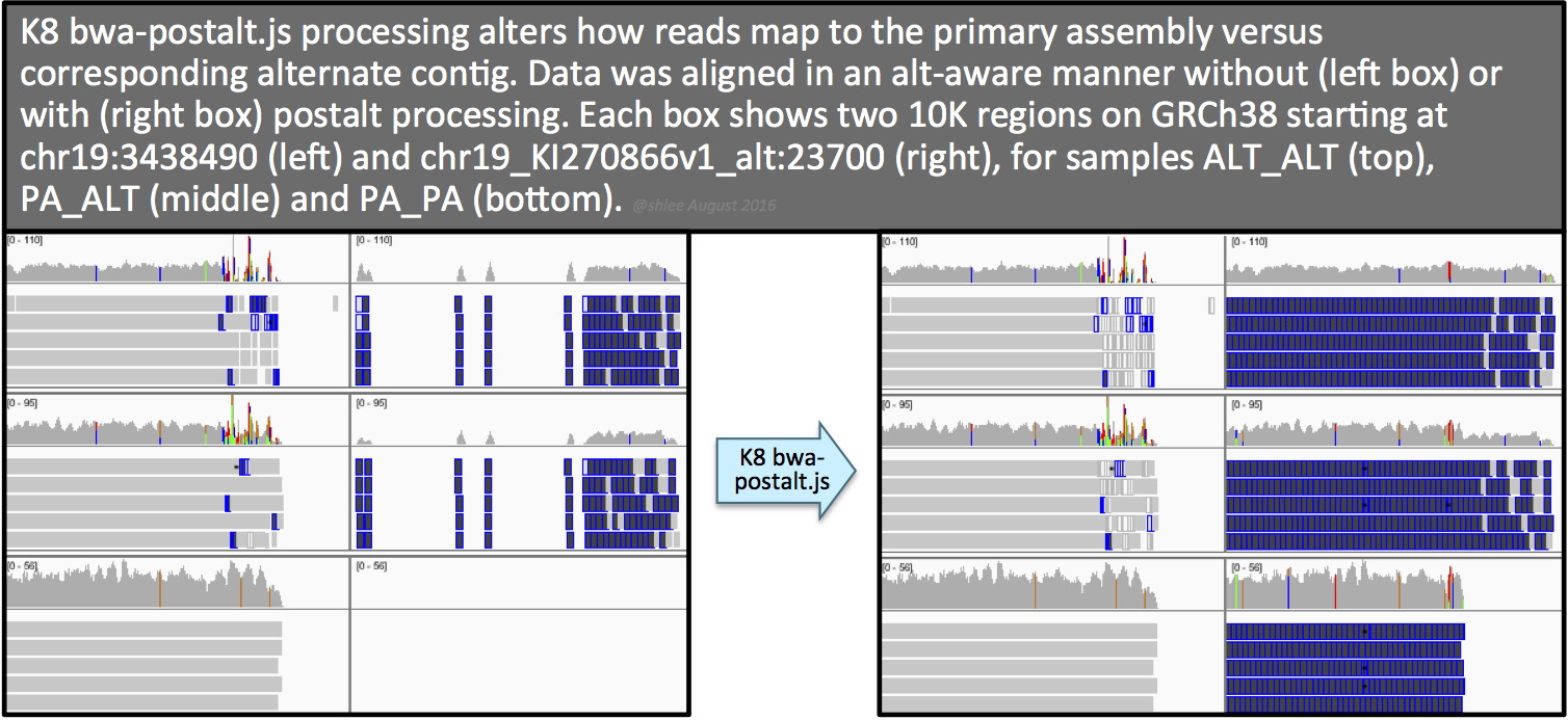
The effect of this postalt-processing is immediately apparent in the IGV screenshots. Previously empty regions are now filled with alignments. Look closely in the highly divergent region of the primary locus. Do you notice a change, albeit subtle, before and after postalt-processing for samples ALTALT and PAALT?
These alignments give the calls below for our SNP sites of interest. Here, notice calls are made for more sites--on the equivalent site if present in addition to the design site (highlighted in the first two columns). For the three pairs of sites that can be called on either the primary locus or alternate contig, the variant site QUALs, the INFO field annotation metrics and the sample level annotation values are identical for each pair.
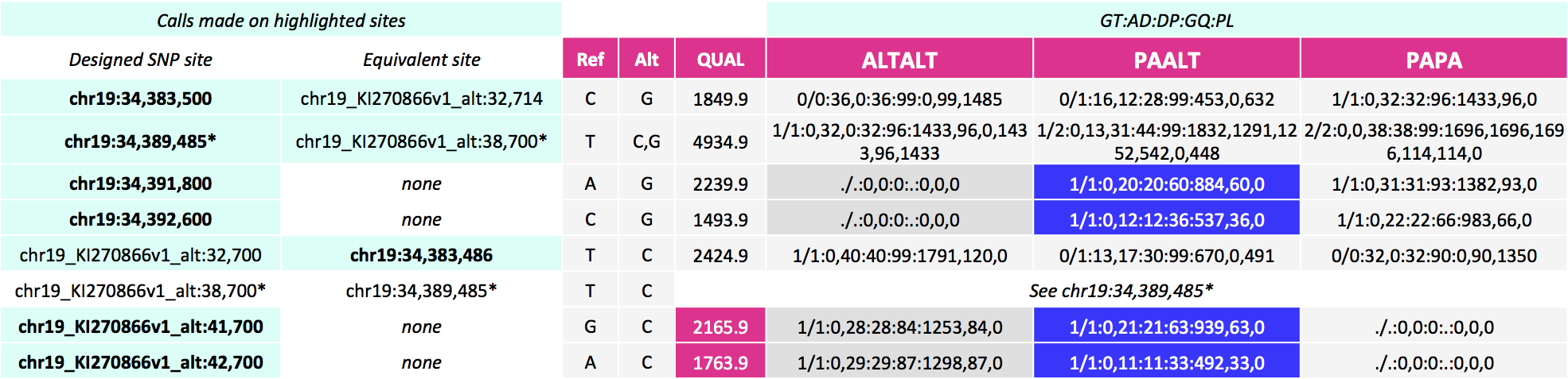
Postalt-processing lowers the MAPQ of primary locus alignments in the highly divergent region that map better to the alt locus. You can see this as a subtle change in the IGV screenshot. After postalt-processing we see an increase in white zero MAPQ reads in the highly divergent region of the primary locus for ALTALT and PAALT. For ALTALT, this effectively cleans up the variant calls in this region at chr19:34,391,800 and chr19:34,392,600. Previously for ALTALT, these calls contained some reads: 4 and 25 for the first workflow and 0 and 28 for the second workflow. After postalt-processing, no reads are considered in this region giving us ./.:0,0:0:.:0,0,0 calls for both sites.
What we omit from examination are the effects of postalt-processing on decoy contig alignments. Namely, if an alignment on the primary assembly aligns better on a decoy contig, then postalt-processing discounts the alignment on the primary assembly by assigning it a zero MAPQ score.
To wrap up, here are the number of variant sites called for the three workflows. As you can see, this last workflow calls the most variants at 95 variant sites, with 62 on the primary assembly and 33 on the alternate contig.
Workflow                total    on primary assembly    on alternate contig
tutorial_8017           56       54                      2
tutorial_8017_toSE      68       66                      2
tutorial_8017_postalt   95       62                     33
7. Related resources
- For WDL scripts of the workflows represented in this tutorial, see the GATK WDL scripts repository.
- To revert an aligned BAM to unaligned BAM, see Section B of Tutorial#6484.
- To simulate reads from a reference contig, see Tutorial#7859.
- Dictionary entry Reference Genome Components reviews terminology that describe reference genome components.
- The GATK resource bundle provides an analysis set GRCh38 reference FASTA as well as several other related resource files.
- As of this writing (August 8, 2016), the SAM format ALT index file for GRCh38 is available only in the x86_64-linux bwakit download as stated in this bwakit README. The
hs38DH.fa.altfile is in theresource-GRCh38folder. Rename this file's basename to match that of the corresponding reference FASTA. - For more details on MergeBamAlignment features, see Section 3C of Tutorial#6483.
- For details on the PairedEndSingleSampleWorkflow that uses GRCh38, see here.
- See here for VCF specifications.
↧
ApplyRecalibration error, during snps recalibration
GATK 4.0.3.0
Hi,
I have a problem with ApplyRecalibration:
A USER ERROR has occurred: Encountered input variant which isn't found in the input recal file. Please make sure VariantRecalibrator and ApplyRecalibration were run on the same set of input variants. First seen at: [VC Unknown @ chr1:12899 Q75.51 of type=SNP alleles=[A*, C] attr={AC=2, AF=0.040, AN=50, DP=66, ExcessHet=0.0445, FS=0.000, InbreedingCoeff=0.1386, MLEAC=3, MLEAF=0.060, MQ=21.65, QD=25.17, SOR=2.833} GT=[] filters=
Here my pipeline:
1A) "Hard Filtering"
input="0.raw.vcf"
output="1.HF_raw.vcf"
${ph6} --java-options -Xmx25g VariantFiltration --filter-expression 'ExcessHet > 54.69' --filter-name 'ExcessHet' -V ${input} -O ${output}
1A) "Make Sites Only Vcf"
input="1.HF_raw.vcf"
output="2.HFso_raw.vcf"
${ph6} --java-options -Xmx25g MakeSitesOnlyVcf -I ${input} -O ${output}
input="2.HFso_raw.vcf"
output="HFso_indel.recal.vcf"
tranches="indels.IVR.tranches"
2A) "Indels Variant Recalibrator"
${ph6} --java-options -Xmx100g VariantRecalibrator -V ${input} -O ${output} --tranches-file ${tranches} -trust-all-polymorphic -tranche "100.0" -tranche "99.95" -tranche "99.9" -tranche "99.5" -tranche "99.0" -tranche "97.0" -tranche "96.0" -tranche "95.0" -tranche "94.0" -tranche "93.5" -tranche "93.0" -tranche "92.0" -tranche "91.0" -tranche "90.0" -an "FS" -an "ReadPosRankSum" -an "MQRankSum" -an "QD" -an "SOR" -an "DP" -mode INDEL --max-gaussians 4 -resource mills,known=false,training=true,truth=true,prior=12:${sorgsorg}/Mills_and_1000G_gold_standard.indels.hg38.vcf.gz -resource axiomPoly,known=false,training=true,truth=false,prior=10:${sorgsorg}/Axiom_Exome_Plus.genotypes.all_populations.poly.hg38.vcf.gz -resource dbsnp,known=true,training=false,truth=false,prior=2:${sorgsorg}/Homo_sapiens_assembly38.dbsnp138.vcf
2B) "SNPs Variant Recalibrator Create Model"
input="2.HFso_raw.vcf"
output="HFso_snp.recal.vcf"
tranches="snps.SVRM.tranches"
model="snps_model.SVRM.report"
${ph6} --java-options -Xmx125g VariantRecalibrator -V ${input} -O ${output} --tranches-file ${tranches} -trust-all-polymorphic -tranche "100.0" -tranche "99.95" -tranche "99.9" -tranche "99.8" -tranche "99.6" -tranche "99.5" -tranche "99.4" -tranche "99.3" -tranche "99.0" -tranche "98.0" -tranche "97.0" -tranche "90.0" -an "QD" -an "MQRankSum" -an "ReadPosRankSum" -an "FS" -an "MQ" -an "SOR" -an "DP" -mode SNP -sample-every "10" --output-model ${model} --max-gaussians 6 -resource hapmap,known=false,training=true,truth=true,prior=15:${sorgsorg}/hapmap_3.3.hg38.vcf.gz -resource omni,known=false,training=true,truth=true,prior=12:${sorgsorg}/1000G_omni2.5.hg38.vcf.gz -resource 1000G,known=false,training=true,truth=false,prior=10:${sorgsorg}/1000G_phase1.snps.high_confidence.hg38.vcf.gz -resource dbsnp,known=true,training=false,truth=false,prior=7:${sorgsorg}/Homo_sapiens_assembly38.dbsnp138.vcf
2C) "SNPsVariantRecalibrator"
input="2.HFso_raw.vcf"
output="provaoutput.vcf"
tranches="snps.SVR.tranches"
model="snps_model.SVR.report"
${ph6} --java-options -Xmx50g VariantRecalibrator -V ${input} -O ${output} --tranches-file ${tranches} -trust-all-polymorphic -tranche "100.0" -tranche "99.95" -tranche "99.9" -tranche "99.8" -tranche "99.6" -tranche "99.5" -tranche "99.4" -tranche "99.3" -tranche "99.0" -tranche "98.0" -tranche "97.0" -tranche "90.0" -an "QD" -an "MQRankSum" -an "ReadPosRankSum" -an "FS" -an "MQ" -an "SOR" -an "DP" -mode SNP --input-model ${model} --max-gaussians 6 -resource hapmap,known=false,training=true,truth=true,prior=15:${sorgsorg}/hapmap_3.3.hg38.vcf.gz -resource omni,known=false,training=true,truth=true,prior=12:${sorgsorg}/1000G_omni2.5.hg38.vcf.gz -resource 1000G,known=false,training=true,truth=false,prior=10:${sorgsorg}/1000G_phase1.snps.high_confidence.hg38.vcf.gz -resource dbsnp,known=true,training=false,truth=false,prior=7:${sorgsorg}/Homo_sapiens_assembly38.dbsnp138.vcf
2D)"ApplyRecalibration"
input="2.HFso_raw.vcf"
outin="tmp.indel.recalibrated.vcf"
output="2.HFso_recalibrated.vcf"
indelrecal="HFso_indel.recal.vcf"
snprecal="HFso_snp.recal.vcf"
indeltranches="indels.IVR.tranches"
snptranches="snps.SVR.tranches"
${ph6} --java-options -Xmx50g ApplyVQSR -O ${outin} -V ${input} --recal-file ${indelrecal} -tranches-file ${indeltranches} -truth-sensitivity-filter-level "99.7" --create-output-variant-index true -mode INDEL
${ph6} --java-options -Xmx50g ApplyVQSR -O ${output} -V ${outin} --recal-file ${snprecal} -tranches-file ${snptranches} -truth-sensitivity-filter-level "99.7" --create-output-variant-index true -mode SNP
Any suggestion?
In the forum I found only old conversations, no about GATK4, if I'm correct.
Many thanks
↧
↧
(How to) Call somatic mutations using GATK4 Mutect2
Post suggestions and read about updates in the Comments section.
 This tutorial introduces researchers to considerations in somatic short variant discovery using GATK4 Mutect2. Example data are based on a breast cancer cell line and its matched normal cell line derived from blood and are aligned to GRCh38 with post-alt processing [1]. The tutorial focuses on how to call traditional somatic short mutations, as described in Article#11127 and pipelined in GATK v4.0.0.0's mutect2.wdl [2]. The tool and its workflow are in BETA status as of this writing, which means they may undergo changes and are not guaranteed for production.
► For Broad Mutation Calling Best Practices, see FireCloud Article#45055.
Section 1 calls somatic mutations with Mutect2 using all the bells and whistles of the tool. Section 2 outlines how to create the panel of normals resource using the tumor-only mode of Mutect2. Section 3 outlines how to estimate cross-sample contamination. Section 4 shows how to filter the callset with FilterMutectCalls. Unlike GATK3, in GATK4 the somatic calling and filtering functionalities are embodied by separate tools. Section 5 shows an optional filtering step to filter by sequence context artifacts that present with orientation bias, e.g. OxoG artifacts. Section 6 shows how to set up in IGV for manual review. Finally, section 7 provides a brief list of related resources that may be of interest to researchers.
GATK4 Mutect2 is a versatile variant caller that not only is more sensitive than, but is also roughly twice as fast as, HaplotypeCaller's reference confidence mode. Researchers who wish to customize analyses should find the tutorial's descriptions of the multiple levers of Mutect2 in section 1 and descriptions of the tumor-only mode of Mutect2 in section 2 of interest.
Jump to a section
- Call somatic short variants and generate a bamout with Mutect2
☞ 1.1 What are the Mutect2 annotations?
☞ 1.2 What is the impact of disabling the MateOnSameContigOrNoMappedMateReadFilter read filter? - Create a sites-only PoN with CreateSomaticPanelOfNormals
☞ 2.1 The tumor-only mode of Mutect2 is useful outside of pon creation - Estimate cross-sample contamination using GetPileupSummaries and CalculateContamination
☞ 3.1 What if I find high levels of contamination? - Filter for confident somatic calls using FilterMutectCalls
- (Optional) Estimate artifacts with CollectSequencingArtifactMetrics and filter them with FilterByOrientationBias
☞ 5.1 Tally of applied filters for the tutorial data - Set up in IGV to review somatic calls
- Related resources
Tools involved
- GATK v4.0.0.0 is available in a Docker image and as a standalone jar. For the latest release, see the Downloads page. Note that GATK v4.0.0.0 contains Picard tools from release v2.17.2 that are callable with the
gatklaunch script. - Desktop IGV. The tutorial uses v2.3.97.
Download example data
Download tutorial_11136.tar.gz, either from the GoogleDrive or from the ftp site. To access the ftp site, leave the password field blank. If the GoogleDrive link is broken, please let us know. The tutorial also requires the GRCh38 reference FASTA, dictionary and index. These are available from the GATK Resource Bundle. For details on the example data and resources, see [3] and [4].
► The tutorial steps switch between the subset and full data. Some of the data files, e.g. BAMs, are restricted to a small region of the genome to efficiently pace the tutorial. Other files, e.g. the Mutect2 calls that the tutorial filters, are from the entire genome. The tutorial content was originally developed for the 2017-09 Helsinki workshop and we make the full data files, i.e. the resource files and the BAMs, available at gs://gatk-best-practices/somatic-hg38.
1. Call somatic short variants and generate a bamout with Mutect2
Here we have a rather complex command to call somatic variants on the HCC1143 tumor sample using Mutect2. For a synopsis of what somatic calling entails, see Article#11127. The command calls somatic variants in the tumor sample and uses a matched normal, a panel of normals (PoN) and a population germline variant resource.
gatk --java-options "-Xmx2g" Mutect2 \
-R hg38/Homo_sapiens_assembly38.fasta \
-I tumor.bam \
-I normal.bam \
-tumor HCC1143_tumor \
-normal HCC1143_normal \
-pon resources/chr17_pon.vcf.gz \
--germline-resource resources/chr17_af-only-gnomad_grch38.vcf.gz \
--af-of-alleles-not-in-resource 0.0000025 \
--disable-read-filter MateOnSameContigOrNoMappedMateReadFilter \
-L chr17plus.interval_list \
-O 1_somatic_m2.vcf.gz \
-bamout 2_tumor_normal_m2.bam
This produces a raw unfiltered somatic callset 1_somatic_m2.vcf.gz, a reassembled reads BAM 2_tumor_normal_m2.bam and the respective indices 1_somatic_m2.vcf.gz.tbi and 2_tumor_normal_m2.bai.
Comments on select parameters
- Specify the case sample for somatic calling with two parameters. Provide the BAM with
-Iand the sample's read group sample name (theSMfield value) with-tumor. To look up the read groupSMfield use GetSampleName. Alternatively, usesamtools view -H tumor.bam | grep '@RG'. - Prefilter variant sites in a control sample alignment. Specify the control BAM with
-Iand the control sample's read group sample name (theSMfield value) with-normal. In the case of a tumor with a matched normal control, we can exclude even rare germline variants and individual-specific artifacts. If we analyze our tumor sample with Mutect2 without the matched normal, we get an order of magnitude more calls than with the matched normal. - Prefilter variant sites in a panel of normals callset. Specify the panel of normals (PoN) VCF with
-pon. Section 2 outlines how to create a PoN. The panel of normals not only represents common germline variant sites, it presents commonly noisy sites in sequencing data, e.g. mapping artifacts or other somewhat random but systematic artifacts of sequencing. By default, the tool does not reassemble nor emit variant sites that match identically to a PoN variant. To enable genotyping of PoN sites, use the--genotype-pon-sitesoption. If the match is not exact, e.g. there is an allele-mismatch, the tool reassembles the region, emits the calls and annotates matches in the INFO field withIN_PON. - Annotate variant alleles by specifying a population germline resource with
--germline-resource. The germline resource must contain allele-specific frequencies, i.e. it must contain the AF annotation in the INFO field [4]. The tool annotates variant alleles with the population allele frequencies. When using a population germline resource, consider adjusting the--af-of-alleles-not-in-resourceparameter from its default of 0.001. For example, the gnomAD resourceaf-only-gnomad_grch38.vcf.gzrepresents ~200k exomes and ~16k genomes and the tutorial data is exome data, so we adjust--af-of-alleles-not-in-resourceto 0.0000025 which corresponds to 1/(2*exome samples). The default of 0.001 is appropriate for human sample analyses without any population resource. It is based on the human average rate of heterozygosity. The population allele frequencies (POP_AF) and theaf-of-alleles-not-in-resourcefactor in probability calculations of the variant being somatic. - Include reads whose mate maps to a different contig. For our somatic analysis that uses alt-aware and post-alt processed alignments to GRCh38, we disable a specific read filter with
--disable-read-filter MateOnSameContigOrNoMappedMateReadFilter. This filter removes from analysis paired reads whose mate maps to a different contig. Because of the way BWA crisscrosses mate information for mates that align better to alternate contigs (in alt-aware mapping to GRCh38), we want to include these types of reads in our analysis. Otherwise, we may miss out on detecting SNVs and indels associated with alternate haplotypes. Disabling this filter deviates from current production practices. - Target the analysis to specific genomic intervals with the
-Lparameter. Here we specify this option to speed up our run on the small tutorial data. For the full callset we use in section 4, calling was on the entirety of the data, without an intervals file. - Generate the reassembled alignments file with
-bamout. The bamout alignments contain the artificial haplotypes and reassembled alignments for the normal and tumor and enable manual review of calls. The parameter is not required by the tool but is recommended as adding it costs only a small fraction of the total run time.
To illustrate how Mutect2 applies annotations, below are five multiallelic sites from the full callset. Pull these out with gzcat somatic_m2.vcf.gz | awk '$5 ~","'. The awk '$5 ~","' subsets records that contain a comma in the 5th column.

We see eleven columns of information per variant call including genotype calls for the normal and tumor. Notice the empty fields for QUAL and FILTER, and annotations at the site (INFO) and sample level (columns 10 and 11). The samples each have genotypes and when a site is multiallelic, we see allele-specific annotations. Samples may have additional annotations, e.g. PGT and PID that relate to phasing.
☞ 1.1 What are the Mutect2 annotations?
We can view the standard FORMAT-level and INFO-level Mutect2 annotations in the VCF header.


The Variant Annotations section of the Tool Documentation further describe some of the annotations. For a complete list of annotations available in GATK4, see this site.
To enable specific filtering that relies on nonstandard annotations, or just to add additional annotations, use the -A argument. For example, -A ReferenceBases adds the ReferenceBases annotation to variant calls. Note that if an annotation a filter relies on is absent, FilterMutectCalls will skip the particular filtering without any warning messages.
☞ 1.2 What is the impact of disabling the MateOnSameContigOrNoMappedMateReadFilter read filter?
To understand the impact, consider some numbers. After all other read filters, the MateOnSameContigOrNoMappedMateReadFilter (MOSCO) filter additionally removes from analysis 8.71% (8,681,271) tumor sample reads and 8.18% (6,256,996) normal sample reads from the full data. The impact of disabling the MOSCO filter is that reads on alternate contigs and read pairs that span contigs can now lend support to variant calls.
For the tutorial data, including reads normally filtered by the MOSCO filter roughly doubles the number of Mutect2 calls. The majority of the additional calls comes from the ALT, HLA and decoy contigs.
2. Create a sites-only PoN with CreateSomaticPanelOfNormals
We make the motions of creating a PoN using three germline samples. These samples are HG00190, NA19771 and HG02759 [3].
First, run Mutect2 in tumor-only mode on each normal sample. In tumor-only mode, a single case sample is analyzed with the -tumor flag without an accompanying matched control -normal sample. For the tutorial, we run this command only for sample HG00190.
gatk Mutect2 \
-R ~/Documents/ref/hg38/Homo_sapiens_assembly38.fasta \
-I HG00190.bam \
-tumor HG00190 \
--disable-read-filter MateOnSameContigOrNoMappedMateReadFilter \
-L chr17plus.interval_list \
-O 3_HG00190.vcf.gz
This generates a callset 3_HG00190.vcf.gz and a matching index. Mutect2 calls variants in the sample with the same sensitive criteria it uses for calling mutations in the tumor in somatic mode. Because the command omits the use of options that trigger upfront filtering, we expect all detectable variants to be called. The calls will include low allele fraction variants and sites with multiple variant alleles, i.e. multiallelic sites. Here are two multiallelic records from 3_HG00190.vcf.gz.

We see for each site, Mutect2 calls the ref allele and three alternate alleles. The GT genotype call is 0/1/2/3. The AD allele depths are 16,3,12,4 and 41,5,24,4, respectively for the two sites.
Comments on select parameters
- One option that is not used here is to include a germline resource with
--germline-resource. Remember from section 1 this resource must containAFpopulation allele frequencies in the INFO column. Use of this resource in tumor-only mode, just as in somatic mode, allows upfront filtering of common germline variant alleles. This effectively omits common germline variant alleles from the PoN. Note the related optional parameter--max-population-af(default 0.01) defines the cutoff for allele frequencies. Given a resource, and read evidence for the variant, Mutect2 will still emit variant alleles withAFless than or equal to the--max-population-af. - Recapitulate any special options used in somatic calling in the panel of normals sample calling, e.g.
--disable-read-filter MateOnSameContigOrNoMappedMateReadFilter. This particular option is relevant for alt-aware and post-alt processed alignments.
Second, collate all the normal VCFs into a single callset with CreateSomaticPanelOfNormals. For the tutorial, to illustrate the step with small data, we run this command on three normal sample VCFs. The general recommendation for panel of normals is a minimum of forty samples.
gatk CreateSomaticPanelOfNormals \
-vcfs 3_HG00190.vcf.gz \
-vcfs 4_NA19771.vcf.gz \
-vcfs 5_HG02759.vcf.gz \
-O 6_threesamplepon.vcf.gz
This generates a PoN VCF 6_threesamplepon.vcf.gz and an index. The tutorial PoN contains 8,275 records.
CreateSomaticPanelOfNormals retains sites with variants in two or more samples. It retains the alleles from the samples but drops all other annotations to create an eight-column, sites-only VCF as shown.

Ideally, the PoN includes samples that are technically representative of the tumor case sample--i.e. samples sequenced on the same platform using the same chemistry, e.g. exome capture kit, and analyzed using the same toolchain. However, even an unmatched PoN will be remarkably effective in filtering a large proportion of sequencing artifacts. This is because mapping artifacts and polymerase slippage errors occur for pretty much the same genomic loci for short read sequencing approaches.
What do you think of including samples of family members in the PoN?
☞ 2.1 The tumor-only mode of Mutect2 is useful outside of pon creation
For example, consider variant calling on data that represents a pool of individuals or a collective of highly similar but distinct DNA molecules, e.g. mitochondrial DNA. Mutect2 calls multiple variants at a site in a computationally efficient manner. Furthermore, the tumor-only mode can be co-opted to simply call differences between two samples. This approach is described in Blog#11315.
3. Estimate cross-sample contamination using GetPileupSummaries and CalculateContamination.
First, run GetPileupSummaries on the tumor BAM to summarize read support for a set number of known variant sites. Use a population germline resource containing only common biallelic variants, e.g. subset by using SelectVariants --restrict-alleles-to BIALLELIC, as well as population AF allele frequencies in the INFO field [4]. The tool tabulates read counts that support reference, alternate and other alleles for the sites in the resource.
gatk GetPileupSummaries \
-I tumor.bam \
-V resources/chr17_small_exac_common_3_grch38.vcf.gz \
-O 7_tumor_getpileupsummaries.table
This produces a six-column table as shown. The alt_count is the count of reads that support the ALT allele in the germline resource. The allele_frequency corresponds to that given in the germline resource. Counts for other_alt_count refer to reads that support all other alleles.

Comments on select parameters
- The tool only considers homozygous alternate sites in the sample that have a population allele frequency that ranges between that set by
--minimum-population-allele-frequency(default 0.01) and--maximum-population-allele-frequency(default 0.2). The rationale for these settings is as follows. If the homozygous alternate site has a rare allele, we are more likely to observe the presence of REF or other more common alleles if there is cross-sample contamination. This allows us to measure contamination more accurately. - One option to speed up analysis, that is not used in the command above, is to limit data collection to a sufficiently large but subset genomic region with the
-Largument.
Second, estimate contamination with CalculateContamination. The tool takes the summary table from GetPileupSummaries and gives the fraction contamination. This estimation informs downstream filtering by FilterMutectCalls.
gatk CalculateContamination \
-I 7_tumor_getpileupsummaries.table \
-O 8_tumor_calculatecontamination.table
This produces a table with estimates for contamination and error. The estimate for the full tumor sample is shown below and gives a contamination fraction of 0.0205. Going forward, we know to suspect calls with less than ~2% alternate allele fraction.

Comments on select parameters
- CalculateContamination can operate in two modes. The command above uses the mode that simply estimates contamination for a given sample. The alternate mode incorporates the metrics for the matched normal, to enable a potentially more accurate estimate. For the second mode, run GetPileupSummaries on the normal sample and then provide the normal pileup table to CalculateContamination with the
-matchedargument.
► Cross-sample contamination differs from normal contamination of tumor and tumor contamination of normal. Currently, the workflow does not account for the latter type of purity issue.
☞ 3.1 What if I find high levels of contamination?
One thing to rule out is sample swaps at the read group level.
Picard’s CrosscheckFingerprints can detect sample-swaps at the read group level and can additionally measure how related two samples are. Because sequencing can involve multiplexing a sample across lanes and regrouping a sample’s multiple read groups, depending on the level of automation in handling these, there is a possibility of including read groups from unrelated samples. The inclusion of such a cross-sample in the tumor sample would be detrimental to a somatic analysis. Without getting into details, the tool allows us to (i) check at the sample level that our tumor and normal are related, as it is imperative they should come from the same individual and (ii) check at the read group level that each of the read group data come from the same individual.
Again, imagine if we mistook the contaminating read group data as some tumor subpopulation! The tutorial normal and tumor samples consist of 16 and 22 read groups respectively, and when we provide these and set EXPECT_ALL_GROUPS_TO_MATCH=true, CrosscheckReadGroupFingerprints (a tool now replaced by CrosscheckFingerprints) informs us All read groups related as expected.
4. Filter for confident somatic calls using FilterMutectCalls
FilterMutectCalls determines whether a call is a confident somatic call. The tool uses the annotations within the callset and applies preset thresholds that are tuned for human somatic analyses.
Filter the Mutect2 callset with FilterMutectCalls. Here we use the full callset, somatic_m2.vcf.gz. To activate filtering based on the contamination estimate, provide the contamination table with --contamination-table. In GATK v4.0.0.0, the tool uses the contamination estimate as a hard cutoff.
gatk FilterMutectCalls \
-V somatic_m2.vcf.gz \
--contamination-table tumor_calculatecontamination.table \
-O 9_somatic_oncefiltered.vcf.gz
This produces a VCF callset 9_somatic_oncefiltered.vcf.gz and index. Calls that are likely true positives get the PASS label in the FILTER field, and calls that are likely false positives are labeled with the reason(s) for filtering in the FILTER field of the VCF. We can view the available filters in the VCF header using grep '##FILTER'.

This step seemingly applies 14 filters, including contamination. However, if an annotation a filter relies on is absent, the tool skips the particular filtering. The filter will still appear in the header. For example, the duplicate_evidence filter requires a nonstandard annotation that our callset omits.
So far, we have 3,695 calls, of which 2,966 are filtered and 729 pass as confident somatic calls. Of the filtered, contamination filters eight calls, all of which would have been filtered for other reasons. For the statistically inclined, this may come as a surprise. However, remember that the great majority of contaminant variants would be common germline alleles, for which we have in place other safeguards.
► In the next GATK version, FilterMutectCalls will use a statistical model to filter based on the contamination estimate.
5. (Optional) Estimate artifacts with CollectSequencingArtifactMetrics and filter them with FilterByOrientationBias
FilterByOrientationBias allows filtering based on sequence context artifacts, e.g. OxoG and FFPE. This step is optional and if employed, should always be performed after filtering with FilterMutectCalls. The tool requires the pre_adapter_detail_metrics from Picard CollectSequencingArtifactMetrics.
First, collect metrics on sequence context artifacts with CollectSequencingArtifactMetrics. The tool categorizes these as those that occur before hybrid selection (preadapter) and those that occur during hybrid selection (baitbias). Results provide a global view across the genome that empowers decision making in ways that site-specific analyses cannot. The metrics can help decide whether to consider downstream filtering.
gatk CollectSequencingArtifactMetrics \
-I tumor.bam \
-O 10_tumor_artifact \
–-FILE_EXTENSION ".txt" \
-R ~/Documents/ref/hg38/Homo_sapiens_assembly38.fasta
Alternatively, use the tool from a standalone Picard jar.
java -jar picard.jar \
CollectSequencingArtifactMetrics \
I=tumor.bam \
O=10_tumor_artifact \
FILE_EXTENSION=.txt \
R=~/Documents/ref/hg38/Homo_sapiens_assembly38.fasta
This generates five metrics files, including pre_adapter_detail_metrics, which contains counts that FilterByOrientationBias uses. Below are the summary pre_adapter_summary_metrics for the full data. Our samples were not from FFPE so we do not expect this artifact. However, it appears that we could have some OxoG transversions.


Picard metrics are described in detail here. For the purposes of this tutorial, we focus on the TOTAL_QSCORE.
- The TOTAL_QSCORE is Phred-scaled such that lower scores equate to a higher probability the change is artifactual. E.g. forty translates to 1 in 10,000 probability. For OxoG, a rough cutoff for concern is 30. FilterByOrientationBias uses the quality score as a prior that a context will produce an artifact. The tool also weighs the evidence from the reads. For example, if the QSCORE is 50 but the allele is supported by 15 reads in F1R2 and no reads in F2R1, then the tool should filter the call.
- FFPE stands for formalin-fixed, paraffin-embedded. Formaldehyde deaminates cytosines and thereby results in C→T transition mutations. Oxidation of guanine to 8-oxoguanine results in G→T transversion mutations during library preparation. Another Picard tool, CollectOxoGMetrics, similarly gives Phred-scaled scores for the 16 three-base extended sequence contexts. In GATK4 Mutect2, the
F1R2andF2R1annotations count the reads in the pair orientation supporting the allele(s). This is a change from GATK3’sFOXOG(fraction OxoG) annotation.
Second, perform orientation bias filtering with FilterByOrientationBias. We provide the tool with the once-filtered calls 9_somatic_oncefiltered.vcf.gz, the pre_adapter_detail_metrics file and the sequencing contexts for FFPE (C→T transition) and OxoG (G→T transversion). The tool knows to include the reverse complement contexts.
gatk FilterByOrientationBias \
-A G/T \
-A C/T \
-V 9_somatic_oncefiltered.vcf.gz \
-P tumor_artifact.pre_adapter_detail_metrics.txt \
-O 11_somatic_twicefiltered.vcf.gz
This produces a VCF 11_somatic_twicefiltered.vcf.gz, index and summary 11_somatic_twicefiltered.vcf.gz.summary. In the summary, we see the number of calls for the sequence context and the number of those that the tool filters.

Is the filtering in line with our earlier prediction?
In the VCF header, we see the addition of the 15th filter, orientation_bias, which the tool applies to 56 calls. All 56 of these calls were previously PASS sites, i.e. unfiltered. We now have 673 passing calls out of 3,695 total calls.

☞ 5.1 Tally of applied filters for the tutorial data
The table shows the breakdown in filters applied to 11_somatic_twicefiltered.vcf.gz. The middle column tallys the instances in which each filter was applied across the calls and the third column tallys the instances in which a filter was the sole reason for a site not passing. Of the total calls, ~18% (673/3,695) are confident somatic calls. Of the filtered calls, ~56% (1,694/3,022) are filtered singly. We see an average of ~1.73 filters per filtered call (5,223/3,022).

Which filters appear to have the greatest impact? What types of calls do you think compels manual review?
Examine passing records with the following command. Take note of the AD and AF annotation values in particular, as they show the high sensitivity of the caller.
gzcat 11_somatic_twicefiltered.vcf.gz | grep -v '#' | awk '$7=="PASS"' | less
6. Set up in IGV to review somatic calls
Deriving a good somatic callset involves comparing callsets, e.g. from different callers or calling approaches, manually reviewing passing and filtered calls and, if necessary, combining callsets and additional filtering. Manual review extends from deciphering call record annotations to the nitty-gritty of reviewing read alignments using a visualizer.
To manually review calls, use the feature-rich desktop version of the Integrative Genomics Viewer (IGV). Remember that Mutect2 makes calls on reassembled alignments that do not necessarily reflect that of the starting BAM. Given this, viewing the raw BAM is insufficient for understanding calls. We must examine the bamout that Mutect2's graph-assembly produces.
First, load Human (hg38) as the reference in IGV. Then load these six files in order:
- resources/chr17_pon.vcf.gz
- resources/chr17_af-only-gnomad_grch38.vcf.gz
- 11_somatic_twicefiltered.vcf.gz
- 2_tumor_normal_m2.bam
- normal.bam
- tumor.bam
With the exception of the somatic callset 11_somatic_twicefiltered.vcf.gz, the subset regions the data cover are in chr17plus.interval_list.
 Second, navigate IGV to the TP53 locus (chr17:7,666,402-7,689,550).
- One of the tracks is dominating the view. Right-click on track
chr17_af-only-gnomad_grch38.vcf.gzand collapse its view. ![image]() Zoom into the somatic call in
Zoom into the somatic call in 11_somatic_twicefiltered.vcf.gz, the gray rectangle in exon 3, by click-dragging on the ruler.- Hover over or click on the gray call in track
11_somatic_twicefiltered.vcf.gzto view INFO level annotations. Similarly, the blue call underneath gives HCC1143_tumor sample level information. - Scroll through the alignment data and notice the coverage for the samples.

A
C→Tvariant is intumor.bambut notnormal.bam. What is happening in2_tumor_normal_m2.bam?
 Third, tweak IGV settings that aid in visualizing reassembled alignments.
- Make room to focus on track
2_tumor_normal_m2.bam. Shift+select on the left panels for trackstumor.bam,normal.bamand their coverages. Right-click and Remove Tracks. - Go to View>Preferences>Alignments. Toggle on Show center line and toggle off Downsample reads.
- Drag the alignments panel to center the red variant.
Right-click on the alignments track and
- Group by sample
- Sort by base
- Color by tag: HC.
Scroll to take note of the number of groups. Click on a read in each group to determine which group belongs to which sample.

What are the three grouped tracks for the bamout? What does the pastel versus gray colors indicate? How plausible is it that all tumor copies of this locus have this alteration?
Here is the corresponding VCF record. Remember Mutect2 makes no ploidy assumption. The GT field tabulates the presence for each allele starting with the reference allele.

| CHROM | POS | ID | REF | ALT | QUAL | FILTER | INFO |
|---|---|---|---|---|---|---|---|
| chr17 | 7,674,220 | . | C | T | . | PASS | DP=122;ECNT=1;NLOD=13.54;N_ART_LOD=-1.675e+00;POP_AF=2.500e-06;P_GERMLINE=-1.284e+01;TLOD=257.15 |
| FORMAT | GT:AD:AF:F1R2:F2R1:MBQ:MFRL:MMQ:MPOS:OBAM:OBAMRC:OBF:OBP:OBQ:OBQRC:SA_MAP_AF:SA_POST_PROB |
|---|---|
| HCC1143_normal | 0/0:45,0:0.032:19,0:26,0:0:151,0:0:0:false:false |
| HCC1143_tumor | 0/1:0,70:0.973:0,34:0,36:33:0,147:60:21:true:false:0.486:0.00:46.01:100.00:0.990,0.990,1.00:0.028,0.026,0.946 |
Finally, here are the indel calls for which we have bamout alignments. All 17 of these happen to be filtered. Explore a few of these sites in IGV to practice the motions of setting up for manual review and to study the logic behind different filters.
| CHROM | POS | REF | ALT | FILTER |
|---|---|---|---|---|
| chr17 | 4,539,344 | T | TA | artifact_in_normal;germline_risk;panel_of_normals |
| chr17 | 7,221,420 | CACTGCCCTAGGTCAGGA | C | artifact_in_normal;panel_of_normals;str_contraction |
| chr17 | 7,483,063 | A | AC | mapping_quality;t_lod |
| chr17 | 8,513,688 | GTT | G | panel_of_normals |
| chr17 | 19,748,387 | G | GA | t_lod |
| chr17 | 26,982,033 | G | GC | artifact_in_normal;clustered_events |
| chr17 | 30,059,463 | CT | C | t_lod |
| chr17 | 35,422,473 | C | CA | t_lod |
| chr17 | 35,671,734 | CTT | C,CT,CTTT | artifact_in_normal;multiallelic;panel_of_normals |
| chr17 | 43,104,057 | CA | C | artifact_in_normal;germline_risk;panel_of_normals |
| chr17 | 43,104,072 | AAAAAAAAAGAAAAG | A | panel_of_normals;t_lod |
| chr17 | 46,332,538 | G | GT | artifact_in_normal;panel_of_normals |
| chr17 | 47,157,394 | CAA | C | panel_of_normals;t_lod |
| chr17 | 50,124,771 | GCACACACACACACACA | G | clustered_events;panel_of_normals;t_lod |
| chr17 | 68,907,890 | GA | G | artifact_in_normal;base_quality;germline_risk;panel_of_normals;t_lod |
| chr17 | 69,182,632 | C | CA | artifact_in_normal;t_lod |
| chr17 | 69,182,835 | GAAAA | G | panel_of_normals |
7. Related resources
The next step after generating a carefully manicured somatic callset is typically functional annotation.
- Funcotator is available in BETA and can annotate GRCh38 and prior reference aligned VCF format data.
- Oncotator can annotate GRCh37 and prior reference aligned MAF and VCF format data. It is also possible to download and install the tool following instructions in Article#4154.
- Annotate with the external program VEP to predict phenotypic changes and confirm or hypothesize biochemical effects.
For a cohort, after annotation, use MutSig to discover driver mutations. MutsigCV (the version is CV) is available on GenePattern. If more samples are needed to increase the power of the analysis, consider padding the analysis set with TCGA Project or other data.
The dSKY plot at https://figshare.com/articles/D_SKY_for_HCC1143/2056665 shows somatic copy number alterations for the HCC1143 tumor sample. Its colorful results remind us that calling SNVs and indels is only one part of cancer genome analyses. Somatic copy number alteration detection will be covered in another GATK tutorial. For reference implementations of Somatic CNV workflows see here.
Footnotes
[1] Data was alt-aware aligned to GRCh38 and post-alt processed. For an introduction to alt-aware alignment and post-alt processing, see [Blog#8180](https://software.broadinstitute.org/gatk/blog?id=8180). The HCC1143 alignments are identical to that in [Tutorial#9183](https://software.broadinstitute.org/gatk/documentation/article?id=9183), which uses GATK3 MuTect2.
[2] For scripted GATK Best Practices Somatic Short Variant Discovery workflows, see [https://github.com/gatk-workflows](https://github.com/gatk-workflows). Within the repository, as of this writing, [gatk-somatic-snvs-indels](https://github.com/gatk-workflows/gatk4-somatic-snvs-indels), which uses GRCh37, is the sole GATK4 Mutect2 workflow. This tutorial uses additional parameters not used in the [GRCh37 gatk-somatic-snvs-indels](https://github.com/gatk-workflows/gatk4-somatic-snvs-indels) example because the tutorial data was preprocessed with post-alt processing of alt-aware alignments, which deviates from production practices. The general workflow steps remain the same.
[3] About the tutorial data:
- The data tarball contains 15 files in the main directory, six files in its resources folder and twenty files in its precomputed folder. Of the files, chr17 refers to data subset to that in the regions in
chr17plus.interval_list, the m2pon consists of forty 1000 Genomes Project samples, pon to panel of normals, tumor to the tumor HCC1143 breast cancer sample and normal to its matched blood normal. - Again, example data are based on a breast cancer cell line and its matched normal cell line derived from blood. Both cell lines are consented and known as HCC1143 and HCC1143_BL, respectively. The Broad Cancer Genome Analysis (CGA) group has graciously provided 2x76 paired-end whole exome sequence data from the two cell lines (C835.HCC1143_2 and C835.HCC1143_BL.4), and @shlee reverted and aligned these to GRCh38 using alt-aware alignment and post-alt processing as described in Tutorial#8017. During preprocessing, the MergeBamAlignment step was omitted, reads containing adapter sequence were removed altogether for both samples (~0.153% of reads in the tumor) as determined by MarkIlluminaAdapters, base qualities were not binned during base recalibration and indel realignment was included to match the toolchain of the PoN normals. The program group for base recalibration is absent from the BAM headers due to a bug in the version of PrintReads at the time of pre-processing, in January of 2017.
- Note that the tutorial uses exome data for its small size. The workflow is applicable to whole genome sequence data (WGS).
- @shlee lifted-over or remapped the gnomAD resource files from GRCh37 counterparts to GRCh38. The tutorial uses subsets of the full resources; the full-length versions are available at gs://gatk-best-practices/somatic-hg38/. The official GRCh37 versions of the resources are available in the GATK Resource Bundle and are based on the gnomAD resource. These GRCh37 versions were prepared by @davidben according to the method outlined in the mutect_resources.wdl and described in [4].
- The full data in the tutorial were generated by @shlee using the github.com/broadinstitute/gatk mutect2.wdl from between the v4.0.0.0 and v4.0.0.1 release with commit hash
b4d1ddd. The GATK Docker image wasbroadinstitute/gatk:4.0.0.0and Picard was v2.14.1. A single modification was made to the script to enable generating the bamout. The script was run locally on a Google Cloud Compute VM using Cromwell v30.1. Given Docker was installed and the specified Docker images were present on the VM, Cromwell automatically launched local Docker container instances during the run and handled the local files as hard-links to avoid redundant copying. Workflow input variables were as follows.
{
  "##_COMMENT1:": "WORKFLOW STEP OPTIONS",
  "Mutect2.is_run_oncotator": "False",
  "Mutect2.is_run_orientation_bias_filter": "True",
  "Mutect2.picard": "/home/shlee/picard-2.14.1.jar",
  "Mutect2.gatk_docker": "broadinstitute/gatk:4.0.0.0",
  "Mutect2.oncotator_docker": "broadinstitute/oncotator:1.9.3.0",
...
  "##_COMMENT3:": "ANALYSIS PARAMETERS",
  "Mutect2.artifact_modes": ["G/T", "C/T"],
  "Mutect2.m2_extra_args": "--af-of-alleles-not-in-resource 0.0000025 --disable-read-filter MateOnSameContigOrNoMappedMateReadFilter",
  "Mutect2.m2_extra_filtering_args": "",
  "Mutect2.scatter_count": "10"
}
- If using newer versions of the
mutect2.wdlthat allow setting SplitIntervals optional arguments, then @shlee recommends setting--subdivision-mode BALANCING_WITHOUT_INTERVAL_SUBDIVISIONto avoid splitting contigs. - With the exception of the PoN and Picard tool steps, data was generated using v4.0.0.0. The PoN was generated using GATK4 vbeta.6. Besides the syntax, little changed for the Mutect2 workflow between these releases and the workflow and most of its tools remain in beta status as of this writing. We used Picard v2.14.1 for the CollectSequencingArtifactMetrics step. Figures in section 5 reflect results from Picard v2.11.0, which give, at glance, identical results as 2.14.1.
- The three samples in section 2 are present in the forty sample PoN used in section 1 and they are 1000 Genomes Project samples.
[4] The WDL script [mutect_resources.wdl](https://github.com/broadinstitute/gatk/blob/master/scripts/mutect2_wdl/mutect_resources.wdl) takes a large gnomAD VCF or other typical cohort VCF and from it prepares both a simplified germline resource for use in _section 1_ and a common biallelic variants resource for use in _section 3_. The script first generates a sites-only VCF and in the process _removes all extraneous annotations_ except for `AF` allele frequencies. We recommend this simplification as the unburdened VCF allows Mutect2 to run much more efficiently. To generate the common biallelic variants resource, the script then selects the biallelic sites from the sites-only VCF.
↧
Ensembl GRCh38 indels and dsnp vcf files
Hello,
I am using GATK3.8 to call variants in RNA-seq data. I am following the best practices for RNA-seq (https://software.broadinstitute.org/gatk/documentation/article.php?id=3891). My problem is during the indel realignment and base calibration steps. I have used the Ensembl GRCh38 genome version to map the reads. The indels and dsnp vcf files I can download from the resource bundle (hg38) have different chromosome notation and contig names (In my bam file chromosomes contain just number, ie "1", and in the vcf the format is "chr1"). Is there any indels and dsnp vcf files with the chromosome notation for Ensembl ? I can change the chromosome format in the vcf files but I dont know if this can be a problem in the next steps of the workflow.
Thanks
Sam
↧
Population frequency in MuTect2
I am running MuTect2 with GATK4 in tumor only mode but the SNPs in my vcfs are not labelled with their rs number or population frequency. Here is the command I am using.
gatk Mutect2 \
-L intervalfile.bed \
-R ucsc.hg19.fasta \
-I sample.bam \
-tumor sampleid \
--germline-resource dbsnp_138.hg19.vcf \
-ip 20 \
-O variants.vcf
CHROM   REF ALT ID  TLOD    AC  FILTER  POS         POP_AF
chr4    A   G   .   3458.76 NA  PASS    55946081    5.000e-08
chr4    A   G   .   2806.25 NA  PASS    55948108    5.000e-08
chr4    A   C   .   1399.17 NA  PASS    55968053    5.000e-08
If I use the GATK VariantAnnotator I am able to get rs number but the population frequency shows up as 5E-8 (even with --resource-allele-concordence set to true). Why is MuTect2 (and VariantAnnotator) not labelling rs number and pop frequency?
gatk VariantAnnotator \
-V variants.vcf\
-O annotatedVariants.vcf \
--dbsnp dbsnp_138.hg19.vcf \
--resourceMills_and_1000G_gold_standard.indels.hg19.sites.vcf \
--resource 1000G_phase1.snps.high_confidence.hg19.sites.vcf \
--resource-allele-concordance true
CHROM   REF ALT ID           TLOD   AC  FILTER  POS         POP_AF
chr4    A   G   rs4421048   3458.76 NA  PASS    55946081    5.000e-08
chr4    A   G   rs2412617   2806.25 NA  PASS    55948108    5.000e-08
chr4    A   C   rs7655964   1399.17 NA  PASS    55968053    5.000e-08
↧
Increase marker or point size for PlotDenoisedCopyRatios?
Is it possible to increase the data marker size for PlotDenoisedCopyRatios? The markers are rather small and difficult to visualize when plotting data where the coverage isn't very dense.
↧
↧
CollectSequencingArtifactMetrics PreAdapterDetailMetrics question
Dear GATK support,
I'm trying to figure out how the error_rate and qscore is calculated in the Picard sequencing artifact metrics. I notice that in the PreAdapterDetailMetrics, for two reverse compliment context, the pro and con ref bases and alt bases are exact opposite, which lead to one to be scored 100 and the other in the 30s. And I got confused now are the pro_ref_bases and con_ref_bases generated? Shouldn't they be the same because they are just reverse comp copy of each other? Example shown below.
REF_BASE ALT_BASE CONTEXT PRO_REF_BASES PRO_ALT_BASES CON_REF_BASES CON_ALT_BASES ERROR_RATE QSCORE
C T TCT 33803861 34212 33838997 62648 0 100
G A AGA 33838997 62648 33803861 34212 0.00042 34
Another related question is, is there any guideline that we can use as recommended cutoff score to define whether a certain base change is artifact instead of true variant?
Thanks,
Wen
↧
SelectVariants tool crashed because of error for input string.
Hi,
I am trying to use GATK's SelectVariants tool to select variants of a specific sample from a vcf file that has variants for 476 different samples (it's a very large file, 14Gb). I have done this before for smaller vcf files and never had any problems. I wonder if it's the vcf file size that is causing the problem.
I'm using java 1.8.0_151.
Here is the command I ran:
java -d64 -Xmx4g -jar /home/tjs23/apps/GenomeAnalysisTK-3.7/GenomeAnalysisTK.jar \
-T SelectVariants \
-R /data2/genome_builds/c_elegans_WS264/c_elegans.PRJNA13758.WS264.genomic.fa \
-V /scratch/gnelson/strain_bbmap/merged_476_comb_freebayes.vcf \
-o /scratch/gnelson/strain_bbmap/AX3841_homozy_freebayes.vcf \
-sn sample_AX3841 \
-select "vc.getGenotype('sample_AX3841').isHomVar()"
Here is the error message:
INFO 12:19:37,470 HelpFormatter - --------------------------------------------------------------------------------
INFO 12:19:37,472 HelpFormatter - The Genome Analysis Toolkit (GATK) v3.7-0-gcfedb67, Compiled 2016/12/12 11:21:18
INFO 12:19:37,472 HelpFormatter - Copyright (c) 2010-2016 The Broad Institute
INFO 12:19:37,473 HelpFormatter - For support and documentation go to https://software.broadinstitute.org/gatk
INFO 12:19:37,473 HelpFormatter - [Thu May 24 12:19:37 BST 2018] Executing on Linux 4.4.0-53-generic amd64
INFO 12:19:37,473 HelpFormatter - OpenJDK 64-Bit Server VM 1.8.0_151-8u151-b12-0ubuntu0.16.04.2-b12
INFO 12:19:37,475 HelpFormatter - Program Args: -T SelectVariants -R /data2/genome_builds/c_elegans_WS264/c_elegans.PRJNA13758.WS264.genomic.fa -V /scratch/gnelson/strain_bbmap/merged_476_comb_freebayes.vcf -o /scratch/gnelson/strain_bbmap/AX3841_homozy_freebayes.vcf -sn sample_AX3841 -select vc.getGenotype('sample_AX3841').isHomVar()
INFO 12:19:37,478 HelpFormatter - Executing as paulafp@mario-xeon on Linux 4.4.0-53-generic amd64; OpenJDK 64-Bit Server VM 1.8.0_151-8u151-b12-0ubuntu0.16.04.2-b12.
INFO 12:19:37,479 HelpFormatter - Date/Time: 2018/05/24 12:19:37
INFO 12:19:37,479 HelpFormatter - --------------------------------------------------------------------------------
INFO 12:19:37,479 HelpFormatter - --------------------------------------------------------------------------------
INFO 12:19:37,494 GenomeAnalysisEngine - Strictness is SILENT
INFO 12:19:37,564 GenomeAnalysisEngine - Downsampling Settings: Method: BY_SAMPLE, Target Coverage: 1000
ERROR --
ERROR stack trace
java.lang.NumberFormatException: For input string: "-IV"
at sun.misc.FloatingDecimal.readJavaFormatString(FloatingDecimal.java:2043)
at sun.misc.FloatingDecimal.parseDouble(FloatingDecimal.java:110)
at java.lang.Double.parseDouble(Double.java:538)
at htsjdk.variant.variantcontext.GenotypeLikelihoods.parseDeprecatedGLString(GenotypeLikelihoods.java:260)
at htsjdk.variant.variantcontext.GenotypeLikelihoods.fromGLField(GenotypeLikelihoods.java:90)
at htsjdk.variant.vcf.AbstractVCFCodec.createGenotypeMap(AbstractVCFCodec.java:715)
at htsjdk.variant.vcf.AbstractVCFCodec$LazyVCFGenotypesParser.parse(AbstractVCFCodec.java:129)
at htsjdk.variant.variantcontext.LazyGenotypesContext.decode(LazyGenotypesContext.java:158)
at htsjdk.variant.vcf.AbstractVCFCodec.parseVCFLine(AbstractVCFCodec.java:348)
at htsjdk.variant.vcf.AbstractVCFCodec.decodeLine(AbstractVCFCodec.java:280)
at htsjdk.variant.vcf.AbstractVCFCodec.decode(AbstractVCFCodec.java:258)
at htsjdk.variant.vcf.AbstractVCFCodec.decode(AbstractVCFCodec.java:61)
at htsjdk.tribble.AsciiFeatureCodec.decode(AsciiFeatureCodec.java:74)
at htsjdk.tribble.AsciiFeatureCodec.decode(AsciiFeatureCodec.java:36)
at htsjdk.tribble.AbstractFeatureCodec.decodeLoc(AbstractFeatureCodec.java:43)
at htsjdk.tribble.index.IndexFactory$FeatureIterator.readNextFeature(IndexFactory.java:508)
at htsjdk.tribble.index.IndexFactory$FeatureIterator.next(IndexFactory.java:470)
at htsjdk.tribble.index.IndexFactory.createIndex(IndexFactory.java:344)
at htsjdk.tribble.index.IndexFactory.createDynamicIndex(IndexFactory.java:307)
at org.broadinstitute.gatk.utils.refdata.tracks.RMDTrackBuilder.createIndexInMemory(RMDTrackBuilder.java:441)
at org.broadinstitute.gatk.utils.refdata.tracks.RMDTrackBuilder.loadIndex(RMDTrackBuilder.java:327)
at org.broadinstitute.gatk.utils.refdata.tracks.RMDTrackBuilder.getFeatureSource(RMDTrackBuilder.java:264)
at org.broadinstitute.gatk.utils.refdata.tracks.RMDTrackBuilder.createInstanceOfTrack(RMDTrackBuilder.java:153)
at org.broadinstitute.gatk.engine.datasources.rmd.ReferenceOrderedQueryDataPool.(ReferenceOrderedDataSource.java:208)
at org.broadinstitute.gatk.engine.datasources.rmd.ReferenceOrderedDataSource.(ReferenceOrderedDataSource.java:88)
at org.broadinstitute.gatk.engine.GenomeAnalysisEngine.getReferenceOrderedDataSources(GenomeAnalysisEngine.java:1052)
at org.broadinstitute.gatk.engine.GenomeAnalysisEngine.initializeDataSources(GenomeAnalysisEngine.java:829)
at org.broadinstitute.gatk.engine.GenomeAnalysisEngine.execute(GenomeAnalysisEngine.java:287)
at org.broadinstitute.gatk.engine.CommandLineExecutable.execute(CommandLineExecutable.java:123)
at org.broadinstitute.gatk.utils.commandline.CommandLineProgram.start(CommandLineProgram.java:256)
at org.broadinstitute.gatk.utils.commandline.CommandLineProgram.start(CommandLineProgram.java:158)
at org.broadinstitute.gatk.engine.CommandLineGATK.main(CommandLineGATK.java:108)
ERROR ------------------------------------------------------------------------------------------
ERROR A GATK RUNTIME ERROR has occurred (version 3.7-0-gcfedb67):
ERROR
ERROR This might be a bug. Please check the documentation guide to see if this is a known problem.
ERROR If not, please post the error message, with stack trace, to the GATK forum.
ERROR Visit our website and forum for extensive documentation and answers to
ERROR commonly asked questions https://software.broadinstitute.org/gatk
ERROR
ERROR MESSAGE: For input string: "-IV"
ERROR ------------------------------------------------------------------------------------------
I have tried to find where the string "-IV" is in the file by using grep. Unfortunately, I could find it. I have also selected random samples of the original vcf file and the command worked fine for those.
Please let me know if you need me to provide any further details.
Many thanks,
Paula
↧
Phased Heterozygous SNP
Dear all,
I have difficulties in understanding the genotypes of the phased SNPs. Here i have a SNP where only one read has a reference allele and 11 reads have an alternate allele and is called as heterozygous SNP.
 chr15  8485088 .   G   T   4936.33 PASS
 BaseQRankSum=1.82;ClippingRankSum=0;ExcessHet=0;FS=2.399;InbreedingCoeff=0.721;
 MQ=60;MQRankSum=0;QD=32.86;ReadPosRankSum=0.267;SOR=1.167;
 DP=10789;AF=0.013;MLEAC=13;MLEAF=0.012;AN=1300;AC=28
GT:AD:DP:GQ:PGT:PID:PL  0/1:1,12:13:3:0|1:8485088_G_T:485,0,3
The genotype for a single sample from a multi-sample VCF is shown here. Could someone throw light on how to interpret the genotype as heterozygous as only one read has reference allele. It should have been called as homozygous SNP. Is this a bug or am i missing something also IGV does not show the reference read.(GATK Version=3.7-0-gcfedb67).
↧
Base Quality Score Recalibration (BQSR)
BQSR stands for Base Quality Score Recalibration. In a nutshell, it is a data pre-processing step that detects systematic errors made by the sequencer when it estimates the quality score of each base call. This document starts with a high-level overview of the purpose of this method; deeper technical are provided further down.
Note that this base recalibration process (BQSR) should not be confused with variant recalibration (VQSR), which is a sophisticated filtering technique applied on the variant callset produced in a later step. The developers who named these methods wish to apologize sincerely to any Spanish-speaking users who might get awfully confused at this point.
Wait, what are base quality scores again?
These scores are per-base estimates of error emitted by the sequencing machines; they express how confident the machine was that it called the correct base each time. For example, let's say the machine reads an A nucleotide, and assigns a quality score of Q20 -- in Phred-scale, that means it's 99% sure it identified the base correctly. This may seem high, but it does mean that we can expect it to be wrong in one case out of 100; so if we have several billion basecalls (we get ~90 billion in a 30x genome), at that rate the machine would make the wrong call in 900 million bases. In practice each basecall gets its own quality score, determined through some dark magic jealously guarded by the manufacturer of the sequencer.
Variant calling algorithms rely heavily on the quality score assigned to the individual base calls in each sequence read. This is because the quality score tells us how much we can trust that particular observation to inform us about the biological truth of the site where that base aligns. If we have a basecall that has a low quality score, that means we're not sure we actually read that A correctly, and it could actually be something else. So we won't trust it as much as other base calls that have higher qualities. In other words we use that score to weigh the evidence that we have for or against a variant allele existing at a particular site.
Okay, so what is base recalibration?
Unfortunately the scores produced by the machines are subject to various sources of systematic (non-random) technical error, leading to over- or under-estimated base quality scores in the data. Some of these errors are due to the physics or the chemistry of how the sequencing reaction works, and some are probably due to manufacturing flaws in the equipment.
Base quality score recalibration (BQSR) is a process in which we apply machine learning to model these errors empirically and adjust the quality scores accordingly. For example we can identify that, for a given run, whenever we called two A nucleotides in a row, the next base we called had a 1% higher rate of error. So any base call that comes after AA in a read should have its quality score reduced by 1%. We do that over several different covariates (mainly sequence context and position in read, or cycle) in a way that is additive. So the same base may have its quality score increased for one reason and decreased for another.
This allows us to get more accurate base qualities overall, which in turn improves the accuracy of our variant calls. To be clear, we can't correct the base calls themselves, i.e. we can't determine whether that low-quality A should actually have been a T -- but we can at least tell the variant caller more accurately how far it can trust that A. Note that in some cases we may find that some bases should have a higher quality score, which allows us to rescue observations that otherwise may have been given less consideration than they deserve. Anecdotally my impression is that sequencers are more often over-confident than under-confident, but we do occasionally see runs from sequencers that seemed to suffer from low self-esteem.
Fantastic! How does it work?
The base recalibration process involves two key steps: first the program builds a model of covariation based on the data and a set of known variants, then it adjusts the base quality scores in the data based on the model. The known variants are used to mask out bases at sites of real (expected) variation, to avoid counting real variants as errors. Outside of the masked sites, every mismatch is counted as an error. The rest is mostly accounting.
There is an optional but highly recommended step that involves building a second model and generating before/after plots to visualize the effects of the recalibration process. This is useful for quality control purposes.
More detailed information
Detailed information about command line options for BaseRecalibrator can be found here.
The tools in this package recalibrate base quality scores of sequencing-by-synthesis reads in an aligned BAM file. After recalibration, the quality scores in the QUAL field in each read in the output BAM are more accurate in that the reported quality score is closer to its actual probability of mismatching the reference genome. Moreover, the recalibration tool attempts to correct for variation in quality with machine cycle and sequence context, and by doing so provides not only more accurate quality scores but also more widely dispersed ones. The system works on BAM files coming from many sequencing platforms: Illumina, SOLiD, 454, Complete Genomics, Pacific Biosciences, etc.
This process is accomplished by analyzing the covariation among several features of a base. For example:
- Reported quality score
- The position within the read
- The preceding and current nucleotide (sequencing chemistry effect) observed by the sequencing machine
These covariates are then subsequently applied through a piecewise tabular correction to recalibrate the quality scores of all reads in a BAM file.
For example, pre-calibration a file could contain only reported Q25 bases, which seems good. However, it may be that these bases actually mismatch the reference at a 1 in 100 rate, so are actually Q20. These higher-than-empirical quality scores provide false confidence in the base calls. Moreover, as is common with sequencing-by-synthesis machine, base mismatches with the reference occur at the end of the reads more frequently than at the beginning. Also, mismatches are strongly associated with sequencing context, in that the dinucleotide AC is often much lower quality than TG. The recalibration tool will not only correct the average Q inaccuracy (shifting from Q25 to Q20) but identify subsets of high-quality bases by separating the low-quality end of read bases AC bases from the high-quality TG bases at the start of the read. See below for examples of pre and post corrected values.
The system was designed for (sophisticated) users to be able to easily add new covariates to the calculations. For users wishing to add their own covariate simply look at QualityScoreCovariate.java for an idea of how to implement the required interface. Each covariate is a Java class which implements the org.broadinstitute.sting.gatk.walkers.recalibration.Covariate interface. Specifically, the class needs to have a getValue method defined which looks at the read and associated sequence context and pulls out the desired information such as machine cycle.
Running the tools
BaseRecalibrator
Detailed information about command line options for BaseRecalibrator can be found here.
This GATK processing step walks over all of the reads in my_reads.bam and tabulates data about the following features of the bases:
- read group the read belongs to
- assigned quality score
- machine cycle producing this base
- current base + previous base (dinucleotide)
For each bin, we count the number of bases within the bin and how often such bases mismatch the reference base, excluding loci known to vary in the population, according to dbSNP. After running over all reads, BaseRecalibrator produces a file called my_reads.recal_data.grp, which contains the data needed to recalibrate reads. The format of this GATK report is described below.
Creating a recalibrated BAM
To create a recalibrated BAM you can use GATK's PrintReads with the engine on-the-fly recalibration capability. Here is a typical command line to do so:
java -jar GenomeAnalysisTK.jar \
   -T PrintReads \
   -R reference.fasta \
   -I input.bam \
   -BQSR recalibration_report.grp \
   -o output.bam
After computing covariates in the initial BAM File, we then walk through the BAM file again and rewrite the quality scores (in the QUAL field) using the data in the recalibration_report.grp file, into a new BAM file.
This step uses the recalibration table data in recalibration_report.grp produced by BaseRecalibration to recalibrate the quality scores in input.bam, and writing out a new BAM file output.bam with recalibrated QUAL field values.
Effectively the new quality score is:
- the sum of the global difference between reported quality scores and the empirical quality
- plus the quality bin specific shift
- plus the cycle x qual and dinucleotide x qual effect
Following recalibration, the read quality scores are much closer to their empirical scores than before. This means they can be used in a statistically robust manner for downstream processing, such as SNP calling. In additional, by accounting for quality changes by cycle and sequence context, we can identify truly high quality bases in the reads, often finding a subset of bases that are Q30 even when no bases were originally labeled as such.
Miscellaneous information
- The recalibration system is read-group aware. It separates the covariate data by read group in the recalibration_report.grp file (using @RG tags) and PrintReads will apply this data for each read group in the file. We routinely process BAM files with multiple read groups. Please note that the memory requirements scale linearly with the number of read groups in the file, so that files with many read groups could require a significant amount of RAM to store all of the covariate data.
- A critical determinant of the quality of the recalibation is the number of observed bases and mismatches in each bin. The system will not work well on a small number of aligned reads. We usually expect well in excess of 100M bases from a next-generation DNA sequencer per read group. 1B bases yields significantly better results.
- Unless your database of variation is so poor and/or variation so common in your organism that most of your mismatches are real snps, you should always perform recalibration on your bam file. For humans, with dbSNP and now 1000 Genomes available, almost all of the mismatches - even in cancer - will be errors, and an accurate error model (essential for downstream analysis) can be ascertained.
- The recalibrator applies a "yates" correction for low occupancy bins. Rather than inferring the true Q score from # mismatches / # bases we actually infer it from (# mismatches + 1) / (# bases + 2). This deals very nicely with overfitting problems, which has only a minor impact on data sets with billions of bases but is critical to avoid overconfidence in rare bins in sparse data.
Example pre and post recalibration results
- Recalibration of a lane sequenced at the Broad by an Illumina GA-II in February 2010
- There is a significant improvement in the accuracy of the base quality scores after applying the GATK recalibration procedure


The output of the BaseRecalibrator
- A Recalibration report containing all the recalibration information for the data
Note that the BasRecalibrator no longer produces plots; this is now done by the AnalyzeCovariates tool.
The Recalibration Report
The recalibration report is a [GATKReport](http://gatk.vanillaforums.com/discussion/1244/what-is-a-gatkreport) and not only contains the main result of the analysis, but it is also used as an input to all subsequent analyses on the data. The recalibration report contains the following 5 tables:
- Arguments Table -- a table with all the arguments and its values
- Quantization Table
- ReadGroup Table
- Quality Score Table
- Covariates Table
Arguments Table
This is the table that contains all the arguments used to run BQSRv2 for this dataset. This is important for the on-the-fly recalibration step to use the same parameters used in the recalibration step (context sizes, covariates, ...).
Example Arguments table:
#:GATKTable:true:1:17::;
#:GATKTable:Arguments:Recalibration argument collection values used in this run
Argument                    Value
covariate                   null
default_platform            null
deletions_context_size      6
force_platform              null
insertions_context_size     6
...
Quantization Table
The GATK offers native support to quantize base qualities. The GATK quantization procedure uses a statistical approach to determine the best binning system that minimizes the error introduced by amalgamating the different qualities present in the specific dataset. When running BQSRv2, a table with the base counts for each base quality is generated and a 'default' quantization table is generated. This table is a required parameter for any other tool in the GATK if you want to quantize your quality scores.
The default behavior (currently) is to use no quantization when performing on-the-fly recalibration. You can override this by using the engine argument -qq. With -qq 0 you don't quantize qualities, or -qq N you recalculate the quantization bins using N bins on the fly. Note that quantization is completely experimental now and we do not recommend using it unless you are a super advanced user.
Example Arguments table:
#:GATKTable:true:2:94:::;
#:GATKTable:Quantized:Quality quantization map
QualityScore  Count        QuantizedScore
0                     252               0
1                   15972               1
2                  553525               2
3                 2190142               9
4                 5369681               9
9                83645762               9
...
ReadGroup Table
This table contains the empirical quality scores for each read group, for mismatches insertions and deletions. This is not different from the table used in the old table recalibration walker.
#:GATKTable:false:6:18:%s:%s:%.4f:%.4f:%d:%d:;
#:GATKTable:RecalTable0:
ReadGroup  EventType  EmpiricalQuality  EstimatedQReported  Observations  Errors
SRR032768  D                   40.7476             45.0000    2642683174    222475
SRR032766  D                   40.9072             45.0000    2630282426    213441
SRR032764  D                   40.5931             45.0000    2919572148    254687
SRR032769  D                   40.7448             45.0000    2850110574    240094
SRR032767  D                   40.6820             45.0000    2820040026    241020
SRR032765  D                   40.9034             45.0000    2441035052    198258
SRR032766  M                   23.2573             23.7733    2630282426  12424434
SRR032768  M                   23.0281             23.5366    2642683174  13159514
SRR032769  M                   23.2608             23.6920    2850110574  13451898
SRR032764  M                   23.2302             23.6039    2919572148  13877177
SRR032765  M                   23.0271             23.5527    2441035052  12158144
SRR032767  M                   23.1195             23.5852    2820040026  13750197
SRR032766  I                   41.7198             45.0000    2630282426    177017
SRR032768  I                   41.5682             45.0000    2642683174    184172
SRR032769  I                   41.5828             45.0000    2850110574    197959
SRR032764  I                   41.2958             45.0000    2919572148    216637
SRR032765  I                   41.5546             45.0000    2441035052    170651
SRR032767  I                   41.5192             45.0000    2820040026    198762
Quality Score Table
This table contains the empirical quality scores for each read group and original quality score, for mismatches insertions and deletions. This is not different from the table used in the old table recalibration walker.
#:GATKTable:false:6:274:%s:%s:%s:%.4f:%d:%d:;
#:GATKTable:RecalTable1:
ReadGroup  QualityScore  EventType  EmpiricalQuality  Observations  Errors
SRR032767            49  M                   33.7794          9549        3
SRR032769            49  M                   36.9975          5008        0
SRR032764            49  M                   39.2490          8411        0
SRR032766            18  M                   17.7397      16330200   274803
SRR032768            18  M                   17.7922      17707920   294405
SRR032764            45  I                   41.2958    2919572148   216637
SRR032765             6  M                    6.0600       3401801   842765
SRR032769            45  I                   41.5828    2850110574   197959
SRR032764             6  M                    6.0751       4220451  1041946
SRR032767            45  I                   41.5192    2820040026   198762
SRR032769             6  M                    6.3481       5045533  1169748
SRR032768            16  M                   15.7681      12427549   329283
SRR032766            16  M                   15.8173      11799056   309110
SRR032764            16  M                   15.9033      13017244   334343
SRR032769            16  M                   15.8042      13817386   363078
...
Covariates Table
This table has the empirical qualities for each covariate used in the dataset. The default covariates are cycle and context. In the current implementation, context is of a fixed size (default 6). Each context and each cycle will have an entry on this table stratified by read group and original quality score.
#:GATKTable:false:8:1003738:%s:%s:%s:%s:%s:%.4f:%d:%d:;
#:GATKTable:RecalTable2:
ReadGroup  QualityScore  CovariateValue  CovariateName  EventType  EmpiricalQuality  Observations  Errors
SRR032767            16  TACGGA          Context        M                   14.2139           817      30
SRR032766            16  AACGGA          Context        M                   14.9938          1420      44
SRR032765            16  TACGGA          Context        M                   15.5145           711      19
SRR032768            16  AACGGA          Context        M                   15.0133          1585      49
SRR032764            16  TACGGA          Context        M                   14.5393           710      24
SRR032766            16  GACGGA          Context        M                   17.9746          1379      21
SRR032768            45  CACCTC          Context        I                   40.7907        575849      47
SRR032764            45  TACCTC          Context        I                   43.8286        507088      20
SRR032769            45  TACGGC          Context        D                   38.7536         37525       4
SRR032768            45  GACCTC          Context        I                   46.0724        445275      10
SRR032766            45  CACCTC          Context        I                   41.0696        575664      44
SRR032769            45  TACCTC          Context        I                   43.4821        490491      21
SRR032766            45  CACGGC          Context        D                   45.1471         65424       1
SRR032768            45  GACGGC          Context        D                   45.3980         34657       0
SRR032767            45  TACGGC          Context        D                   42.7663         37814       1
SRR032767            16  AACGGA          Context        M                   15.9371          1647      41
SRR032764            16  GACGGA          Context        M                   18.2642          1273      18
SRR032769            16  CACGGA          Context        M                   13.0801          1442      70
SRR032765            16  GACGGA          Context        M                   15.9934          1271      31
...
Troubleshooting
The memory requirements of the recalibrator will vary based on the type of JVM running the application and the number of read groups in the input bam file.
If the application reports 'java.lang.OutOfMemoryError: Java heap space', increase the max heap size provided to the JVM by adding ' -Xmx????m' to the jvm_args variable in RecalQual.py, where '????' is the maximum available memory on the processing computer.
I've tried recalibrating my data using a downloaded file, such as NA12878 on 454, and apply the table to any of the chromosome BAM files always fails due to hitting my memory limit. I've tried giving it as much as 15GB but that still isn't enough.
All of our big merged files for 454 are running with -Xmx16000m arguments to the JVM -- it's enough to process all of the files. 32GB might make the 454 runs a lot faster though.
I have a recalibration file calculated over the entire genome (such as for the 1000 genomes trio) but I split my file into pieces (such as by chromosome). Can the recalibration tables safely be applied to the per chromosome BAM files?
Yes they can. The original tables needed to be calculated over the whole genome but they can be applied to each piece of the data set independently.
I'm working on a genome that doesn't really have a good SNP database yet. I'm wondering if it still makes sense to run base quality score recalibration without known SNPs.
The base quality score recalibrator treats every reference mismatch as indicative of machine error. True polymorphisms are legitimate mismatches to the reference and shouldn't be counted against the quality of a base. We use a database of known polymorphisms to skip over most polymorphic sites. Unfortunately without this information the data becomes almost completely unusable since the quality of the bases will be inferred to be much much lower than it actually is as a result of the reference-mismatching SNP sites.
However, all is not lost if you are willing to experiment a bit. You can bootstrap a database of known SNPs. Here's how it works:
- First do an initial round of SNP calling on your original, unrecalibrated data.
- Then take the SNPs that you have the highest confidence in and use that set as the database of known SNPs by feeding it as a VCF file to the base quality score recalibrator.
- Finally, do a real round of SNP calling with the recalibrated data. These steps could be repeated several times until convergence.
Downsampling to reduce run time
For users concerned about run time please note this small analysis below showing the approximate number of reads per read group that are required to achieve a given level of recalibration performance. The analysis was performed with 51 base pair Illumina reads on pilot data from the 1000 Genomes Project. Downsampling can be achieved by specifying a genome interval using the -L option. For users concerned only with recalibration accuracy please disregard this plot and continue to use all available data when generating the recalibration table.

↧
↧
VariantRecalibrator - no data found
I just updated to the latest nightly and got the same error:
INFO 12:03:16,652 VariantRecalibratorEngine - Finished iteration 45. Current change in mixture coefficients = 0.00258
INFO 12:03:23,474 ProgressMeter - GL000202.1:10465 5.68e+07 32.4 m 34.0 s 98.7% 32.9 m 25.0 s
INFO 12:03:32,263 VariantRecalibratorEngine - Convergence after 46 iterations!
INFO 12:03:41,008 VariantRecalibratorEngine - Evaluating full set of 4944219 variants...
INFO 12:03:41,100 VariantDataManager - Training with worst 0 scoring variants --> variants with LOD <= -5.0000.
ERROR ------------------------------------------------------------------------------------------
ERROR stack trace
java.lang.IllegalArgumentException: No data found.
at org.broadinstitute.sting.gatk.walkers.variantrecalibration.VariantRecalibratorEngine.generateModel(VariantRecalibratorEngine.java:83)
at org.broadinstitute.sting.gatk.walkers.variantrecalibration.VariantRecalibrator.onTraversalDone(VariantRecalibrator.java:392)
at org.broadinstitute.sting.gatk.walkers.variantrecalibration.VariantRecalibrator.onTraversalDone(VariantRecalibrator.java:138)
at org.broadinstitute.sting.gatk.executive.Accumulator$StandardAccumulator.finishTraversal(Accumulator.java:129)
at org.broadinstitute.sting.gatk.executive.LinearMicroScheduler.execute(LinearMicroScheduler.java:116)
at org.broadinstitute.sting.gatk.GenomeAnalysisEngine.execute(GenomeAnalysisEngine.java:313)
at org.broadinstitute.sting.gatk.CommandLineExecutable.execute(CommandLineExecutable.java:121)
at org.broadinstitute.sting.commandline.CommandLineProgram.start(CommandLineProgram.java:248)
at org.broadinstitute.sting.commandline.CommandLineProgram.start(CommandLineProgram.java:155)
at org.broadinstitute.sting.gatk.CommandLineGATK.main(CommandLineGATK.java:107)
ERROR ------------------------------------------------------------------------------------------
ERROR A GATK RUNTIME ERROR has occurred (version nightly-2014-03-20-g65934ae):
ERROR
ERROR This might be a bug. Please check the documentation guide to see if this is a known problem.
ERROR If not, please post the error message, with stack trace, to the GATK forum.
ERROR Visit our website and forum for extensive documentation and answers to
ERROR commonly asked questions http://www.broadinstitute.org/gatk
ERROR
ERROR MESSAGE: No data found.
ERROR ------------------------------------------------------------------------------------------
↧
Warning messages when perform GenotypeGVCFs
Hi,
I am running a variant calling analysis using GATK 4.0.1.2 suite on 25 human subjects. After I use CombineGVCFs to have a single gvcf file and run GenotypeGVCFs, the log repeatedly shows
WARN InbreedingCoeff - Annotation will not be calculated, must provide at least 10 samples
for several hours. I have opened the combined gvcf from CombineGVCF and confirmed I have all samples in it. For the function arguments, I am using defaults.
Since this repeatedly shows up, I wonder if this is normal.
Thank you very much!
↧
RevertSam per readgroup rather than using OUTPUT_BY_READGROUP
Hi GATK team,
I have been having some troubles implementing RevertSam with OUTPUT_BY_READGROUP set to true due to pipeline software constraints (see that issue here but unrelated to GATK). Suffice to say, I should run a seperate instance of RevertSam for each readgroup.
I tried running the following:
samtools view -br {READGROUP_ID} {SAMPLE_BAM} | gatk RevertSam --INPUT=/dev/stdin --OUTPUT={OUTPUT}
And this seems to work fine (despite being a tad slow). Is there any reason why I should not do it this way?
Thanks!
↧
Performance troubleshooting tips for GenotypeGVCFs
Hi,
I am running a GATK4 variant calling analysis on few hundred Solanum lycopersicum samples via bcbio (species is diploid, 1gigaBase reference) . Everything went fine up to and including importing to the Intel GenomicsDB (GenomicsDBImport) for chromosome region splits. The haplotype caller step just gave warnings about no AVX support.
The GenotypeGVCFs progress however is very slow. Even for very small genome chunks GenotypeGVCFs is not proceeding much let alone finishing. The progress log shows either (almost) no updates or a progress of something like 3 variants per minute. In total I expect to have 100M+ variants.
I am currently running on older hardware without any AVX support. So I am planning to try to run on modern hardware with AVX support to see if that makes a difference.
In the mean while I am wondering if there are other things that I could try to get the analysis to complete.
I noticed that the GenotypeGVCFs was running single threaded and using ca 60+ GB of memory. The -nt multi threading option from GATK3.X does not exist anymore. Is there another option for activating multi threading? And is the 60GB memory normal for few hundred samples?
I tried lowering --max-alternate-alleles from the default of 6 to 4. This did not seem to help.
Do you expect AVX support to make a large difference in performance of GenotypeGVCFs?
In the past I successfully analyzed this data set using Freebayes single batch variant calling. So I don't think this is a data issue.
Is there anything else I could try to fix the performance of GenotypeGVCFs?
Thank you.
P.S.
Here is some log info
[2018-02-18T18:34Z] machine9:     java -Dsamjdk.use_async_io_read_samtools=false -Dsamjdk.use_async_io_write_samtools=true -Dsamjdk.use_async_io_write_tribble=false -Dsamjdk.compression_level=1 -Xms500m -Xmx37265m -XX:+UseSerialGC -Djava.io.tmpdir=/data/run/Projects/DA_1080/DA_1080_bam_tables/work/bcbiotx/tmp7DOD_G -jar /data/prod/Tools/bcbio/1.0.8/anaconda/share/gatk4-4.0.1.1-0/gatk-package-4.0.1.1-local.jar GenotypeGVCFs --variant gendb:///data/run/Projects/DA_1080/DA_1080_bam_tables/work/joint/gatk-haplotype-joint/DA_1080/Chr_00/DA_1080-Chr_00_2336001_2741048_genomicsdb -R /data/prod/Tools/bcbio/1.0.8/genomes/reference/reference/seq/reference.fa --output /data/run/Projects/DA_1080/DA_1080_bam_tables/work/bcbiotx/tmp_bQJhv/DA_1080-Chr_00_2336001_2741048.vcf.gz -L Chr_00:2336002-2741048
[2018-02-18T18:34Z] machine9: 19:34:49.876 INFO  NativeLibraryLoader - Loading libgkl_compression.so from jar:file:/data/prod/Tools/bcbio/1.0.8/anaconda/share/gatk4-4.0.1.1-0/gatk-package-4.0.1.1-local.jar!/com/intel/gkl/native/libgkl_compression.so
[2018-02-18T18:34Z] machine9: 19:34:50.385 INFO  GenotypeGVCFs - ------------------------------------------------------------
[2018-02-18T18:34Z] machine9: 19:34:50.385 INFO  GenotypeGVCFs - The Genome Analysis Toolkit (GATK) v4.0.1.1
[2018-02-18T18:34Z] machine9: 19:34:50.385 INFO  GenotypeGVCFs - For support and documentation go to https://software.broadinstitute.org/gatk/
[2018-02-18T18:34Z] machine9: 19:34:50.386 INFO  GenotypeGVCFs - Executing as ggher@machine9 on Linux v2.6.32-642.4.2.el6.x86_64 amd64
[2018-02-18T18:34Z] machine9: 19:34:50.386 INFO  GenotypeGVCFs - Java runtime: OpenJDK 64-Bit Server VM v1.8.0_121-b15
[2018-02-18T18:34Z] machine9: 19:34:50.386 INFO  GenotypeGVCFs - Start Date/Time: February 18, 2018 7:34:49 PM CET
[2018-02-18T18:34Z] machine9: 19:34:50.386 INFO  GenotypeGVCFs - ------------------------------------------------------------
[2018-02-18T18:34Z] machine9: 19:34:50.386 INFO  GenotypeGVCFs - ------------------------------------------------------------
[2018-02-18T18:34Z] machine9: 19:34:50.388 INFO  GenotypeGVCFs - HTSJDK Version: 2.14.1
[2018-02-18T18:34Z] machine9: 19:34:50.388 INFO  GenotypeGVCFs - Picard Version: 2.17.2
[2018-02-18T18:34Z] machine9: 19:34:50.388 INFO  GenotypeGVCFs - HTSJDK Defaults.COMPRESSION_LEVEL : 1
[2018-02-18T18:34Z] machine9: 19:34:50.388 INFO  GenotypeGVCFs - HTSJDK Defaults.USE_ASYNC_IO_READ_FOR_SAMTOOLS : false
[2018-02-18T18:34Z] machine9: 19:34:50.388 INFO  GenotypeGVCFs - HTSJDK Defaults.USE_ASYNC_IO_WRITE_FOR_SAMTOOLS : true
[2018-02-18T18:34Z] machine9: 19:34:50.388 INFO  GenotypeGVCFs - HTSJDK Defaults.USE_ASYNC_IO_WRITE_FOR_TRIBBLE : false
[2018-02-18T18:34Z] machine9: 19:34:50.389 INFO  GenotypeGVCFs - Deflater: IntelDeflater
[2018-02-18T18:34Z] machine9: 19:34:50.389 INFO  GenotypeGVCFs - Inflater: IntelInflater
[2018-02-18T18:34Z] machine9: 19:34:50.389 INFO  GenotypeGVCFs - GCS max retries/reopens: 20
[2018-02-18T18:34Z] machine9: 19:34:50.389 INFO  GenotypeGVCFs - Using google-cloud-java patch 6d11bef1c81f885c26b2b56c8616b7a705171e4f from https://github.com/droazen/google-cloud-java/tree/dr_all_nio_fixes
[2018-02-18T18:34Z] machine9: 19:34:50.389 INFO  GenotypeGVCFs - Initializing engine
[2018-02-18T18:34Z] machine9: WARNING: No valid combination operation found for INFO field DS - the field will NOT be part of INFO fields in the generated VCF records
[2018-02-18T18:34Z] machine9: WARNING: No valid combination operation found for INFO field InbreedingCoeff - the field will NOT be part of INFO fields in the generated VCF records
[2018-02-18T18:34Z] machine9: WARNING: No valid combination operation found for INFO field MLEAC - the field will NOT be part of INFO fields in the generated VCF records
[2018-02-18T18:34Z] machine9: WARNING: No valid combination operation found for INFO field MLEAF - the field will NOT be part of INFO fields in the generated VCF records
[2018-02-18T18:34Z] machine9: 19:34:51.245 INFO  IntervalArgumentCollection - Processing 405047 bp from intervals
[2018-02-18T18:34Z] machine9: 19:34:51.251 INFO  GenotypeGVCFs - Done initializing engine
[2018-02-18T18:34Z] machine9: 19:34:51.858 INFO  ProgressMeter - Starting traversal
[2018-02-18T18:34Z] machine9: 19:34:51.858 INFO  ProgressMeter -        Current Locus  Elapsed Minutes    Variants Processed  Variants/Minute
[2018-02-18T18:34Z] machine9: WARNING: No valid combination operation found for INFO field DS - the field will NOT be part of INFO fields in the generated VCF records
[2018-02-18T18:34Z] machine9: WARNING: No valid combination operation found for INFO field InbreedingCoeff - the field will NOT be part of INFO fields in the generated VCF records
[2018-02-18T18:34Z] machine9: WARNING: No valid combination operation found for INFO field MLEAC - the field will NOT be part of INFO fields in the generated VCF records
[2018-02-18T18:34Z] machine9: WARNING: No valid combination operation found for INFO field MLEAF - the field will NOT be part of INFO fields in the generated VCF records
[2018-02-18T18:35Z] machine9: 19:35:33.941 INFO  ProgressMeter -       Chr_00:2337001              0.7                  1000           1425.8
[2018-02-18T19:12Z] machine9: 20:12:55.889 INFO  ProgressMeter -       Chr_00:2338001             38.1                  2000             52.5
Here is some typical progress info
[2018-02-18T10:52Z] machine20: 11:52:25.520 INFO  ProgressMeter -        Current Locus  Elapsed Minutes    Variants Processed  Variants/Minute
[2018-02-18T10:52Z] machine20: WARNING: No valid combination operation found for INFO field DS - the field will NOT be part of INFO fields in the generated VCF records
[2018-02-18T10:52Z] machine20: WARNING: No valid combination operation found for INFO field InbreedingCoeff - the field will NOT be part of INFO fields in the generated VCF records
[2018-02-18T10:52Z] machine20: WARNING: No valid combination operation found for INFO field MLEAC - the field will NOT be part of INFO fields in the generated VCF records
[2018-02-18T10:52Z] machine20: WARNING: No valid combination operation found for INFO field MLEAF - the field will NOT be part of INFO fields in the generated VCF records
[2018-02-18T13:37Z] machine16: 14:37:09.060 INFO  ProgressMeter -        Chr_00:879729           1400.7                  1000              0.7
[2018-02-18T13:37Z] machine16: 14:37:54.815 INFO  ProgressMeter -        Chr_00:880729           1401.4                  2000              1.4
[2018-02-18T13:51Z] machine16: 14:51:38.628 INFO  ProgressMeter -        Chr_00:881729           1415.1                  3000              2.1
[2018-02-18T13:53Z] machine16: 14:53:04.278 INFO  ProgressMeter -        Chr_00:884120           1416.6                  5000              3.5
[2018-02-18T13:54Z] machine16: 14:54:12.151 INFO  ProgressMeter -        Chr_00:886120           1417.7                  7000              4.9
↧
↧
Silent failure in CollectAllelicCounts
I'm attempting to do CNV analysis in the latest GATK docker container (4.0.4.0), but have run into a problem at the CollectAllelicCounts stage. The function appears to fail silently after initializing engine. stdout is below:
Using GATK jar /gatk/build/libs/gatk-package-4.0.4.0-local.jar
Running:
    java -Dsamjdk.use_async_io_read_samtools=false -Dsamjdk.use_async_io_write_samtools=true -Dsamjdk.use_async_io_write_tribble=false -Dsamjdk.compression_level=2 -Xmx8g -jar /gatk/build/libs/gatk-package-4.0.4.0-local.jar CollectAllelicCounts -L /refgene/1000G_phase1_omni_hapmap_ENTIRE_dbsnp_146_PADDED_ONLY.interval_list -I /gatk4_test/aligned/CU-03135_S44_L001_001_180426_M05411_0064_000000000-BTHDG.bam -R /refgene/Homo_sapiens_assembly38.fasta -O /gatk4_test/variants/CU-03135_S44_L001_001_180426_M05411_0064_000000000-BTHDG.alleliccounts.tsv
13:46:15.196 INFO  NativeLibraryLoader - Loading libgkl_compression.so from jar:file:/gatk/build/libs/gatk-package-4.0.4.0-local.jar!/com/intel/gkl/native/libgkl_compression.so
13:46:15.524 INFO  CollectAllelicCounts - ------------------------------------------------------------
13:46:15.525 INFO  CollectAllelicCounts - The Genome Analysis Toolkit (GATK) v4.0.4.0
13:46:15.526 INFO  CollectAllelicCounts - For support and documentation go to https://software.broadinstitute.org/gatk/
13:46:15.527 INFO  CollectAllelicCounts - Executing as root@19feeb04fb7d on Linux v4.9.87-linuxkit-aufs amd64
13:46:15.527 INFO  CollectAllelicCounts - Java runtime: OpenJDK 64-Bit Server VM v1.8.0_131-8u131-b11-2ubuntu1.16.04.3-b11
13:46:15.528 INFO  CollectAllelicCounts - Start Date/Time: May 25, 2018 1:46:15 PM UTC
13:46:15.529 INFO  CollectAllelicCounts - ------------------------------------------------------------
13:46:15.530 INFO  CollectAllelicCounts - ------------------------------------------------------------
13:46:15.531 INFO  CollectAllelicCounts - HTSJDK Version: 2.14.3
13:46:15.531 INFO  CollectAllelicCounts - Picard Version: 2.18.2
13:46:15.532 INFO  CollectAllelicCounts - HTSJDK Defaults.COMPRESSION_LEVEL : 2
13:46:15.532 INFO  CollectAllelicCounts - HTSJDK Defaults.USE_ASYNC_IO_READ_FOR_SAMTOOLS : false
13:46:15.532 INFO  CollectAllelicCounts - HTSJDK Defaults.USE_ASYNC_IO_WRITE_FOR_SAMTOOLS : true
13:46:15.533 INFO  CollectAllelicCounts - HTSJDK Defaults.USE_ASYNC_IO_WRITE_FOR_TRIBBLE : false
13:46:15.534 INFO  CollectAllelicCounts - Deflater: IntelDeflater
13:46:15.534 INFO  CollectAllelicCounts - Inflater: IntelInflater
13:46:15.535 INFO  CollectAllelicCounts - GCS max retries/reopens: 20
13:46:15.535 INFO  CollectAllelicCounts - Using google-cloud-java patch 6d11bef1c81f885c26b2b56c8616b7a705171e4f from https://github.com/droazen/google-cloud-java/tree/dr_all_nio_fixes
13:46:15.535 WARN  CollectAllelicCounts -

[1m[31m   !!!!!!!!!!!!!!!!!!!!!!!!!!!!!!!!!!!!!!!!!!!!!!!!!!!!!!!!!!!!

   Warning: CollectAllelicCounts is a BETA tool and is not yet ready for use in production

   !!!!!!!!!!!!!!!!!!!!!!!!!!!!!!!!!!!!!!!!!!!!!!!!!!!!!!!!!!!![0m


13:46:15.536 INFO  CollectAllelicCounts - Initializing engine
Using GATK jar /gatk/build/libs/gatk-package-4.0.4.0-local.jar
The last line is where it starts analyzing the next record, before producing any output. The filenames specified by the -O in my command are never created.
↧
Options GATK4 HaplotypeCaller vs Varscan
I'm new with GATK. I usually use Varscan for variant calling with the following options :
--min-coverage 7 --min-reads2 7 --min-var-freq 0.80 --variants
Which options I have to use with Gatk 4 HaplotypeCaller for similar results?
↧
RevertSam (SANITIZE=TRUE) via pipe leads to SAMException
I am experiencing a similar problem here as previously reported: https://gatkforums.broadinstitute.org/gatk/discussion/10406/strange-revertsam-error
Running
samtools view -br {READGROUP_ID} {SAMPLE_BAM} | gatk RevertSam --INPUT=/dev/stdin --OUTPUT={OUTPUT}
Works fine
Adding additional parameters to RevertSam results in an error:
samtools view -br {READGROUP_ID} {SAMPLE_BAM} | gatk RevertSam --INPUT=/dev/stdin --OUTPUT={OUTPUT} --RESTORE_ORIGINAL_QUALITIES=true --VALIDATION_STRINGENCY=SILENT --ATTRIBUTE_TO_CLEAR=AS --ATTRIBUTE_TO_CLEAR=FT --ATTRIBUTE_TO_CLEAR=CO --ATTRIBUTE_TO_CLEAR=XT --ATTRIBUTE_TO_CLEAR=XN --ATTRIBUTE_TO_CLEAR=OC --ATTRIBUTE_TO_CLEAR=OP --SANITIZE=true --SORT_ORDER=queryname --MAX_DISCARD_FRACTION=0.05

Exception in thread "main" htsjdk.samtools.SAMException: Cannot determine candidate qualities: no qualities found.
I have not tested each parameter individually, but I made the following observations:
samtools view -br {READGROUP_ID} {SAMPLE_BAM} | gatk RevertSam --INPUT=/dev/stdin --OUTPUT={OUTPUT} --RESTORE_ORIGINAL_QUALITIES=true
Works fine
samtools view -br {READGROUP_ID} {SAMPLE_BAM} | gatk RevertSam --INPUT=/dev/stdin --OUTPUT={OUTPUT} --SANITIZE=true
Results in a SAMException
P.S. tests were done using small ~300 kb sized BAM file publicly available, happy to share to easily reproduce error
N.B. using GATK 4.0.2.1
↧